Appendix A
Review of Vectors and Matrices
A.1. Vectors
A.1.1 Definition
For the purposes of this text, a
vector is an object which has magnitude and direction. Examples include forces, electric fields, and
the normal to a surface. A vector is
often represented pictorially as an arrow and symbolically by an underlined
letter or using bold type .
Its magnitude is denoted or .
There are two special cases of vectors: the unit vector has ; and the null vector has .
A.1.2 Vector Operations
Addition
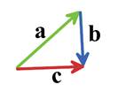
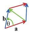
Let and be vectors.
Then is also a vector. The vector may be shown diagramatically by placing arrows
representing and head to tail, as shown below.
Multiplication
1. Multiplication
by a scalar. Let be a vector, and a scalar.
Then is a vector.
The direction of is parallel to and its magnitude is given by .
Note
that you can form a unit vector n which is parallel to a by setting .
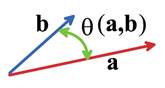
2. Dot Product (also
called the scalar product). Let a
and b be two vectors. The dot product of a and b is a scalar
denoted by , and is defined by
,
where is the angle subtended by a and b, as shown below.
Note that , and .
If and then if and only if ; i.e. a and b are
perpendicular.
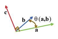
3. Cross Product (also
called the vector product). Let a and b be two vectors. The cross
product of a and b is a vector denoted by . The direction of c is perpendicular to a
and b, and is chosen so that (a,b,c) form a right handed triad, as
shown below.
The magnitude of c is given by
Note that and .
It can sometimes be helpful to
re-write a cross product as a tensor product.
For example, can be re-written as , where
Some useful vector identities
A.1.3 Cartesian components of vectors
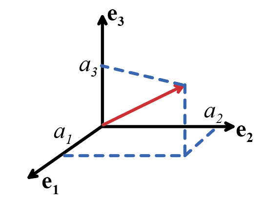 Let be three mutually perpendicular unit vectors
which form a right handed triad, as shown in the figure. Then are said to form and orthonormal basis. The
vectors satisfy
Let be three mutually perpendicular unit vectors
which form a right handed triad, as shown in the figure. Then are said to form and orthonormal basis. The
vectors satisfy
We may express any vector a as a suitable combination of the unit
vectors , and .
For example, we may write
where are scalars, called the components of a in the
basis .
The components of a have a
simple physical interpretation. For
example, if we evaluate the dot product we find that
in view of the properties of the three vectors , and .
Recall that
Then, noting that , we have
Thus, represents the projected length of the vector a
in the direction of , as illustrated in the figure above. Similarly, and may be shown to represent the projection of in the directions and , respectively.
The advantage of representing vectors
in a Cartesian basis is that vector addition and multiplication can be
expressed as simple operations on the components of the vectors. For example, let a, b and c be vectors, with components , and , respectively. Then, it is straightforward to show that
A.1.4 Change of basis
Let a be a vector, and let be a Cartesian basis. Suppose that the components of a in the basis are known to be .
Now, suppose that we wish to compute the components of a in a second Cartesian basis, .
This means we wish to find components , such that
To do so, note that
This transformation is conveniently written as a matrix
operation
,
where is a matrix consisting of the components of a in the basis , is a matrix consisting of the components of a in the basis , and is a ‘rotation matrix’ as follows
Note that the elements of have a simple physical interpretation. For example, , where is the angle between the and axes.
Similarly where is the angle between the and axes.
In practice, we usually know the angles between the axes that make up
the two bases, so it is simplest to assemble the elements of by putting the cosines of the known angles in
the appropriate places.
Index notation provides another convenient way to write this
transformation:
You don’t need to know index notation in detail to understand
this all you need to know is that
The same approach may be used to find
an expression for in terms of .
If you work through the details, you will find that
Comparing this result with the formula for in terms of , we see that
where the superscript T denotes the transpose (rows and
columns interchanged). The transformation matrix is therefore orthogonal, and satisfies
where [I] is the
identity matrix.
A.1.5 Useful vector operations
·  Calculating areas The area of a triangle bounded by vectors a, b¸and
b-a is
Calculating areas The area of a triangle bounded by vectors a, b¸and
b-a is
The area of the parallelogram shown
in the figure is 2A.
· Calculating angles The angle between two vectors a and b is
· Calculating the normal to a surface. If two vectors a and b can be found which are known to lie in the surface, then the unit
normal to the surface is
If the surface is
specified by a parametric equation of the form , where s and t are two
parameters and r is the position
vector of a point on the surface, then two vectors which lie in the plane may
be computed from
· 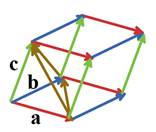 Calculating Volumes The volume of the parallelopiped
defined by three vectors a, b, c
as shown in the figure is
Calculating Volumes The volume of the parallelopiped
defined by three vectors a, b, c
as shown in the figure is
The volume of the
tetrahedron is V/6.
A.2. Vector fields and vector calculus
A.2.1. Scalar field.
Let
be a Cartesian basis with origin O in three
dimensional space. Let
denote the position vector of a point
in space. A scalar field is a scalar valued function of position in space. A scalar field is a function of the
components of the position vector, and so may be expressed as . The value of at a particular point in space must be
independent of the choice of basis vectors.
A scalar field may be a function of time (and possibly other parameters)
as well as position in space.
A.2.2. Vector field
Let
be a Cartesian basis with origin O in three
dimensional space. Let
denote the position vector of a point
in space. A vector field is a vector valued function of position in space. A vector field is a function of the
components of the position vector, and so may be expressed as .
The vector may also be expressed as components in the basis
The magnitude and direction of at a particular point in space is independent
of the choice of basis vectors. A
vector field may be a function of time (and possibly other parameters) as well
as position in space.
A.2.3. Change of basis for scalar fields.
Let be a Cartesian basis with origin O in three
dimensional space, as shown below. Express the position vector of a point
relative to O in as
and let be a scalar field.
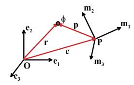
Let be a second Cartesian basis, with origin
P. Let denote the position vector of P relative to O. Express the position vector
of a point relative to P in as
To find , use the following procedure. First, express p as
components in the basis , using the procedure outlined in
Section 1.4:
where
or, using index notation
where the transformation matrix is defined in Sect 1.4. Now, express c as components in , and note that
so that
A.2.4. Change of basis for vector fields.
Let be a Cartesian basis with origin O in three
dimensional space, as shown below.
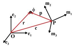
Express the position vector of a
point relative to O in as
and let be a vector
field, with components
Let be a second Cartesian basis, with origin
P. Let denote the position vector of P relative to O. Express the position vector
of a point relative to P in as
To express the vector field as
components in and as a function of the components of p, use the following procedure. First, express in terms of using the procedure outlined for scalar fields
in the preceding section
for k=1,2,3. Now, find the
components of v in using the procedure outlined in Section
1.4. Using index notation, the result is
A.2.5. Time derivatives of vectors
Let a(t) be a vector whose magnitude and direction vary with time, t.
Suppose that is a fixed basis, i.e. independent of
time. We may express a(t)
in terms of components in the basis as
.
The time derivative of a is defined using the usual rules of calculus
,
or in component form as
The definition of the time derivative of a vector may be used
to show the following rules
A.2.6. Using a rotating basis
It is often convenient to express
position vectors as components in a basis which rotates with time. To write equations of motion one must
evaluate time derivatives of rotating vectors.
Let be a basis which rotates with instantaneous
angular velocity .
Then,
A.2.7. Gradient of a scalar field.
Let be a scalar field in three dimensional
space. The gradient of is a vector field denoted by or , and is defined so that
for every position r
in space and for every vector a.
Let be a Cartesian basis with origin O in three
dimensional space. Let
denote the position vector of a point
in space. Express as a function of the components of r .
The gradient of in this basis is then given by
A.2.8. Gradient of a vector field
Let v be a vector field in three dimensional space. The gradient of v is a tensor field denoted by or , and is defined so that
for every position r
in space and for every vector a.
Let be a Cartesian basis with origin O in three dimensional
space. Let
denote the position vector of a point
in space. Express v as a function of the components of r, so that .
The gradient of v in this basis is then given by
Alternatively, in index notation
The gradient can also be taken from the left (but this is
less common). This operation is defined
as
for every position r
in space and for every vector a. Expressed in component form, the left
gradient is
Evidently .
HEALTH WARNING: The notation used for the gradient of a vector is not standard,
unfortunately. Many publications use to denote the gradient taken from the
right.
A.2.9. Divergence of a vector field
Let v be a vector field in three dimensional space. The divergence of v is a scalar field denoted by or .
Formally, it is defined as (the trace of a tensor is the sum of its
diagonal terms).
Let be a Cartesian basis with origin O in three dimensional
space. Let
denote the position vector of a point in space. Express v
as a function of the components of r:
. The divergence of v is then
A.2.10. Curl of a vector field.
Let v be a vector field in three dimensional space. The curl of
v is a vector field denoted by or .
It is best defined in terms of its components in a given basis, although
its magnitude and direction are not dependent on the choice of basis.
Let be a Cartesian basis with origin O in three
dimensional space. Let
denote the position vector of a point
in space. Express v as a function of the components of r . The curl of v
in this basis is then given by
Using index notation, this may be expressed as
A.2.11 The Divergence Theorem.
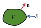 Let V be a closed region in three dimensional space, bounded by an
orientable surface S. Let n denote the unit vector normal to S, taken so that n points out of V as
shown in the figure. Let u be a vector field which is continuous
and has continuous first partial derivatives in some domain containing V.
Then
Let V be a closed region in three dimensional space, bounded by an
orientable surface S. Let n denote the unit vector normal to S, taken so that n points out of V as
shown in the figure. Let u be a vector field which is continuous
and has continuous first partial derivatives in some domain containing V.
Then
alternatively, expressed in index notation
For a proof of this extremely useful theorem consult e.g.
Kreyzig, (1998).
A.3. Matrices
A.3.1 Definition
An matrix is a set of numbers, arranged in m rows and n columns
· A square matrix has equal numbers of rows
and columns
· A diagonal matrix is a square matrix with
elements such that for
· The identity matrix is a diagonal matrix for which all diagonal
elements
· A symmetric matrix is a square matrix
with elements such that
· A skew symmetric matrix is a square
matrix with elements such that
A.3.2 Matrix operations
Addition
Let and be two matrices of order with elements and . Then
Multiplication
· Multiplication by a scalar. Let be a matrix with elements , and let k be a scalar. Then
· Multiplication by a
matrix. Let be a matrix of order with elements , and let be a matrix of order with elements . The product is defined only if n=p, and is an matrix such that
Note that multiplication is distributive and
associative, but not commutative, i.e.
The multiplication
of a vector by a matrix is a particularly important operation. Let b
and c be two vectors with n components, which we think of as matrices.
Let be an matrix.
Thus
Now,
i.e.
Transpose.
Let be a matrix of order with elements . The transpose of is denoted . If is an matrix such that , then , i.e.
Note that
Determinant
The determinant is defined only for a square
matrix. Let be a matrix with components . The determinant of is denoted by or and is given by
Now, let be an matrix.
Define the minors of as the determinant formed by omitting the ith row and jth column of . For example, the minors and for a matrix are computed as follows. Let
Then
Define the cofactors
of as
Then, the determinant of the matrix is computed as follows
The result is the same whichever row i is chosen for the expansion. For the particular case of a matrix
The determinant may also be evaluated by summing over rows,
i.e.
and as before the result is the same for
each choice of column j. Finally, note that
Inversion.
Let be an matrix.
The inverse of is denoted by and is defined such that
The inverse of exists if and only if . A matrix which has no inverse is said to be singular. The inverse of a matrix may be computed
explicitly, by forming the cofactor
matrix with components as defined in the preceding section. Then
In practice, it is faster to compute the
inverse of a matrix using methods such as Gaussian elimination.
Note that
For a diagonal
matrix, the inverse
is
For a matrix, the inverse is
Eigenvalues and
eigenvectors.
Let be an matrix, with coefficients . Consider the vector equation
where x is a vector with n
components, and is a scalar (which may be complex). The n
nonzero vectors x and corresponding
scalars which satisfy this equation are the eigenvectors and eigenvalues of .
Formally, eigenvalues
and eigenvectors may be computed as follows.
Rearrange the preceding equation to
This has nontrivial
solutions for x only if the determinant of the
matrix vanishes.
The equation
is an nth order polynomial which may be solved for .
In general the polynomial will have n
roots, which may be complex. The
eigenvectors may then be computed by finding x satisfying .
For example, a matrix generally has two eigenvectors, which
satisfy
Solve the quadratic equation to see that
The two corresponding eigenvectors may be
computed from (2), which shows that
so that, multiplying
out the first row of the matrix (you can use the second row too, if you wish since we chose to make the determinant of the matrix vanish,
the two equations have the same solutions.
In fact, if , you will need to
do this, because the first equation will simply give 0=0 when trying to solve
for one of the eigenvectors)
which are satisfied by any vector of the
form
where p
and q are arbitrary real numbers.
It is often
convenient to normalize eigenvectors
so that they have unit ‘length’. For
this purpose, choose p and q so that .
(For vectors of dimension n,
the generalized dot product is defined such that )
You can calculate explicit
expressions for eigenvalues and eigenvectors for any matrix up to order , but the results are so cumbersome
that, except for the results, they are virtually useless. In practice, numerical values may be computed
using several iterative techniques. Symbolic
manipulation programs make calculations like this easy.
The eigenvalues of a real symmetric
matrix are always real, and its eigenvectors are orthogonal, i.e. the ith
and jth eigenvectors (with ) satisfy .
The eigenvalues of a skew symmetric matrix are pure
imaginary.
Spectral and singular value decomposition.
Let be a real symmetric matrix. Denote the n (real)
eigenvalues of by , and let be the corresponding normalized eigenvectors, such that . Then, for any arbitrary vector b,
Let be a diagonal matrix which contains the n eigenvalues of as elements of the diagonal, and let be a matrix consisting of the n eigenvectors as columns, i.e.
Then
Note that this gives another (generally quite useless) way to
invert
where is easy to compute since is diagonal.
Square root of a
matrix.
Let be a real symmetric matrix.
Denote the singular value decomposition of by as defined above.
Suppose that denotes the square root of , defined so that
One way to compute is through the singular value decomposition of
where
