10.2 Motion and Deformation of slender rods

 

 

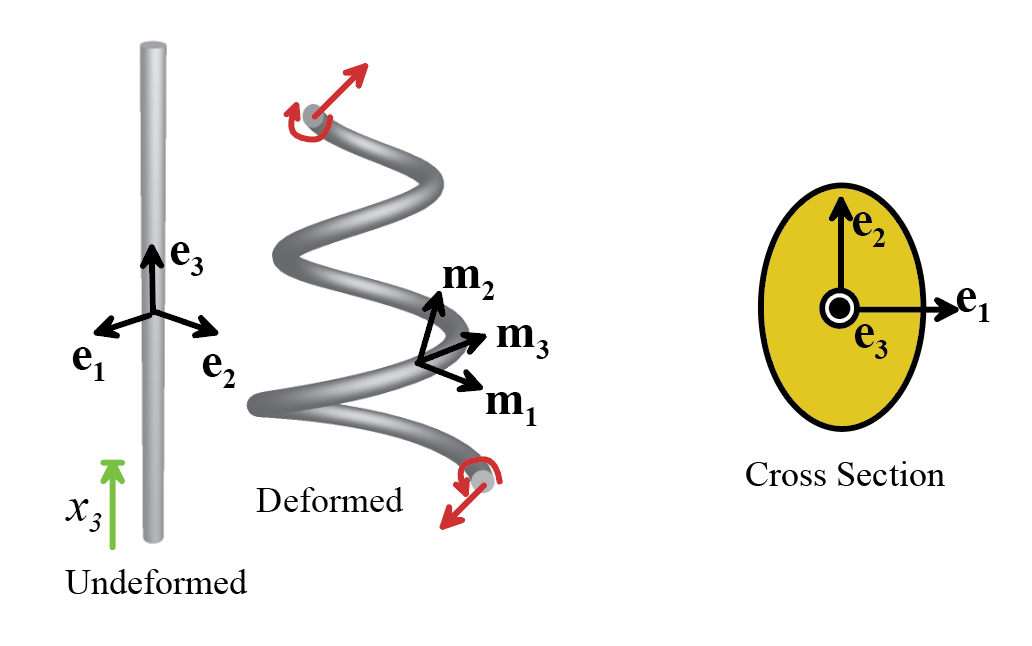
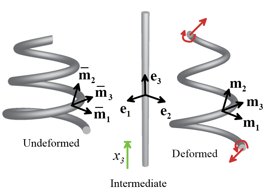
The figure below illustrates the problem to be solved.   We suppose that a long, initially straight rod with length $L_0$ is subjected to forces and moments that cause it to stretch to a new total length L, as well as to bend and twist into a complex three dimensional shape, which we wish to determine.  The initial shape need not necessarily be stress free.  Consequently, we can solve problems involving a rod that is bent and twisted in its unloaded configuration (such as a helical spring) by first mapping it onto an intermediate, straight reference configuration, and then analyzing the deformation of this shape.

 

 

 

 

10.2.1 Variables characterizing the geometry of the rod’s cross-section

 

The figure above illustrates a generic cross-section of the (undeformed) rod. We will characterize the shape of the cross-section as follows:

 

1. We introduce three mutually perpendicular, unit basis vectors $\left\{e_1,e_2,e_3\right\}$, with $e_3$ pointing parallel to the axis of the undeformed cylinder, and $e_1,e_2$ parallel to the principal moments of area of the (undeformed) cross section. 

 

2. We introduce a coordinate system $(x_1,x_2)$ within the cross section, with origin at the centroid of the cross-section.

 

3. The cross-sectional area of the rod is denoted by $A={\displaystyle \underset{A}{\int }d}A$

 

4. The principal moments of area of the cross-section are defined as

$I_1={\displaystyle \underset{A}{\int }{x}_2^{2}dA}{I}_2={\displaystyle \underset{A}{\int }{x}_1^{2}dA}{I}_3={\displaystyle \underset{A}{\int }\left(x_1^2+x_2^2\right)dA}$

 

5. We define a moment of area tensor H for the cross-section, with components $H_{11}=I_1$, $H_{22}=I_2$, $H_{33}=I_3$ and all other components zero.

 

6. In calculations to follow, it will be helpful to note that, because of the choice of origin and coordinate system,

${\displaystyle \underset{A}{\int }{x}_{1}dA}={\displaystyle \underset{A}{\int }{x}_{2}dA}={\displaystyle \underset{A}{\int }{x}_1{x}_{2}dA=0}$

 

Principal moments of area and their directions are listed for a few simple geometries in the table below.  Recall also that area moments of inertia for hollow sections can be calculated by subtraction.

 

 

 

 

10.2.2 Coordinate systems and variables characterizing the deformation of a rod

 

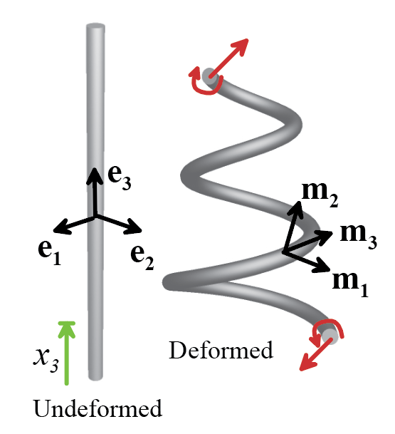A generic twisted rod is illustrated in the figure. The deformation of the rod is described as follows:

 

· The orientation of the straight rod is characterized using the $\left\{e_1,e_2,e_3\right\}$ basis described in the preceding section.

 

· The position vector of a material particle in the reference configuration is $x=x_i{e}_i$, where $x_1=x_2=0$ corresponds to the centroid of the cross section, and $x_3$ is the height above the base of the cylinder.

 

· After deformation, the axis of the cylinder lies on a smooth curve.  The point that lies at $x=x_3{e}_3$ in the undeformed solid moves to a new position $y=r(x_3)$ after deformation.

 

· The orientation of the cross-section after deformation will be described by introducing a basis of mutually perpendicular unit vectors $\left\{m_1,m_2,m_3\right\}$, chosen so that $m_3$ is parallel to the axis of the deformed rod, and is $m_1$ parallel to the line of material points that lay along $e_1$ in the reference configuration (or, more precisely, parallel to the projection of this line perpendicular to $m_3$ ).  Note that the three basis vectors $\left\{m_1,m_2,m_3\right\}$ are all functions of $x_3$, and if the rod is moving, they are also functions of time.

 

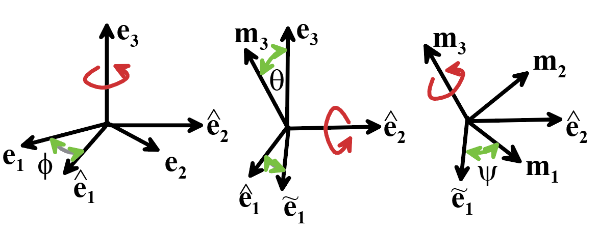
· The orientation of $\left\{m_1,m_2,m_3\right\}$ can be specified by three Euler angles $(\theta ,\varphi ,\psi )$, which characterize the rigid rotation that maps $\left\{e_1,e_2,e_3\right\}$ onto  $\left\{m_1,m_2,m_3\right\}$.   To visualize the significance of the three angles, note that the rotation can be accomplished in three stages, as shown below: (i) rotate the basis vectors through an angle $\varphi$ about the $e_3$ axis.   This results in a new set of vectors $\left\{{\widehat{e}}_1,{\widehat{e}}_2,e_3\right\}$; (ii) Rotate these new vectors through an angle $\theta$ about the ${\widehat{e}}_2$ axis.  This rotates the vectors onto a second configuration $\left\{{\tilde{e}}_1,{\widehat{e}}_2,m_3\right\}$; (iii) finally, rotate these vectors through angle $\psi$ about the $m_3$ direction, to create the $\left\{m_1,m_2,m_3\right\}$ vectors.   

 

 

· Relationships between the Euler angles and the curve characterizing the axis of the rod will be given shortly: these results will show that the angles $\varphi$ and $\theta$ can be determined from the shape of the axis.   The angle $\psi$ is an independent degree of freedom, and quantifies the rotation of the rod’s cross-section about its axis.  

 

· We let $s$ denote the arc length measured along the axis of the rod in the deformed configuration.

 

· The velocity of the rod is characterized by the velocity vector of its axis, $v=dr/dt$

 

· The rate of rotation of the rod is characterized by the angular velocity $\omega ={\omega }_i{m}_i$ of the basis vectors $\left\{m_1,m_2,m_3\right\}$.  It will be shown in Sect 10.2.3 that the angular velocity can be related to the velocity v of the bar’s axis and its twist $\psi$ by

$\omega =m_3\times {\displaystyle \frac{dv}{ds}+\dot{\psi }{m}_3}$

 

· The acceleration of the rod is characterized by the acceleration vector of its axis, $a=dv/dt$

 

· The angular acceleration of the rod is characterized by the angular acceleration $\alpha ={\alpha }_i{m}_i$ of the basis vectors.  It will be shown below that the angular acceleration can be related to the acceleration a and velocity v of the bar’s axis and its twist $\psi$ by

$\alpha ={\displaystyle \frac{d\omega }{dt}=m_3\times {\displaystyle \frac{da}{ds}-2\left({\displaystyle \frac{dv}{ds}\cdot m_3}\right)m_3\times {\displaystyle \frac{dv}{ds}+{\displaystyle \frac{d\psi }{dt}\left\{{\displaystyle \frac{dv}{ds}-\left({\displaystyle \frac{dv}{ds}\cdot m_3}\right)m_3}\right\}+{\displaystyle \frac{d^2\psi }{d{t}^2}{m}_3}}}}}$

 

 

 

10.2.3 Additional deformation measures and useful kinematic relations

 

In this section we introduce some additional measures of the deformation of the rod, as well as several useful relations between the various deformation measures.

 

· The curve corresponding to the axis of the deformed rod is often characterized by its tangent, normal and binormal vectors, together with its curvature, and its torsion.   These are defined as follows.

 

1. The tangent vector $t={\displaystyle \frac{dr}{ds}={\displaystyle \frac{dr}{d{x}_3}{\displaystyle \frac{d{x}_3}{ds}=m_3}}}$

 

2. The normal vector and curvature are defined so that

$\kappa n={\displaystyle \frac{dt}{ds}={\displaystyle \frac{d{m}_3}{d{x}_3}{\displaystyle \frac{d{x}_3}{ds}}}}$,

where n is a unit vector

 

3. The binormal vector is defined as $b=t\times n$

 

4. The triad of unit vectors $\{t,n,b\}$ defines the Frenet Basis for the curve

 

5. The torsion of the curve is defined as $\tau =-n\cdot {\displaystyle \frac{db}{ds}}$.  Note that the torsion is simply a geometric property of the curve $–$ it is not necessarily related to the rod’s twist.

 

These variables are not sufficient to completely describe the deformation, however, since the twist of the rod can vary independently of the shape of its axis.

 

· The two bases $\left\{e_1,e_2,e_3\right\}$, $\left\{m_1,m_2,m_3\right\}$ can be related in terms of the Euler angles as follows.

$\begin{array}{l}{m}_1=\left(\cos \psi \cos \theta \cos \varphi -\sin \psi \sin \varphi \right)e_1+\left(\cos \psi \cos \theta \sin \varphi +\sin \psi \cos \varphi \right)e_2-\cos \psi \sin \theta e_3\\ m_2=-\left(\cos \psi \sin \varphi +\sin \psi \cos \theta \cos \varphi \right)e_1+\left(\cos \psi \cos \varphi -\sin \psi \cos \theta \sin \varphi \right)e_2+\sin \psi \sin \theta e_3\\ m_3=\sin \theta \left(\cos \varphi e_1+\sin \varphi e_2\right)+\cos \theta e_3\end{array}$

These results can be derived by calculating the effects of the sequence of three rotations.  Note also that since both sets of basis vectors are triads of mutually perpendicular unit vectors, they must be related by

$m_i=R{e}_i{e}_i=R^T{m}_i=m_{i}R$

where $R$ is a proper orthogonal tensor that can be visualized as a rigid rotation.   The rotation tensor can be expressed in several different forms:

 

1. It can be expressed as the sum of three dyadic products $R=m_i\otimes e_i$

 

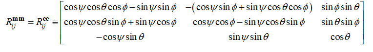
2. It can be expressed as components in either $\left\{e_1,e_2,e_3\right\}$ or $\left\{m_1,m_2,m_3\right\}$, which can be written in dyadic notation as $R_{ij}^{ee}{e}_i\otimes e_j$ or $R_{ij}^{mm}{m}_i\otimes m_j$.  Surprisingly, the components both bases are equal, and are given by $R_{ij}^{mm}=R_{ij}^{ee}=e_i\cdot m_j$. The components can be expressed in terms of the Euler angles as a matrix

 

· In further calculations the variation of basis vectors $m_i$ with distance s along the deformed rod will play a central role.  To visualize this quantity, imagine that the basis $\{m_1,m_2,m_3\}$ travels up the deformed rod. The basis vectors will then rotate with an angular velocity that depends on the curvature and twist of the deformed rod, suggesting that we can characterize the rate of change of orientation with arc-length by a vector $\kappa$, analogous to an angular velocity vector.  The curvature vector can be expressed as components in the basis $\{m_1,m_2,m_3\}$ as $\kappa ={\kappa }_i{m}_i$.  This vector has the following properties

 

1. The curvature vector is (by definition) related to the rate of change of  $m_i$ with s by

${\displaystyle \frac{d{m}_i}{ds}=\kappa \times m_i}$

which can be expanded out to show that

${\displaystyle \frac{d{m}_1}{ds}=-{\kappa }_2{m}_3+{\kappa }_3{m}_2{\displaystyle \frac{d{m}_2}{ds}={\kappa }_1{m}_3-{\kappa }_3{m}_1{\displaystyle \frac{d{m}_3}{ds}=-{\kappa }_1{m}_2+{\kappa }_2{m}_1}}}$

 

2. The components ${\kappa }_1,{\kappa }_2$ quantify the bending of the rod, and are related the curvature $\kappa$ and the binormal vector $b$ of the curve traced by the axis of the deformed rod by ${\kappa }_1{m}_1+{\kappa }_2{m}_2=\kappa b$.  You can show this result by comparing the formula for $d{m}_3/ds$ with the formula for b.

 

3. The curvature vector can also be expressed in terms of the position vector of the rod’s centroid as

${\kappa }_i{m}_i={\displaystyle \frac{dr}{ds}\times {\displaystyle \frac{d^{2}r}{d{s}^2}+{\kappa }_3{\displaystyle \frac{dr}{ds}}}}$

The component of curvature ${\kappa }_3$ cannot in general be expressed in terms of r, because the rotation of the rod’s cross-section about its centroid axis may provide an additional, independent contribution to ${\kappa }_3$.  For the special case where $m_1$ and $m_2$ are everywhere parallel to the normal vector n and binormal b, respectively, it follows that ${\kappa }_3=b\cdot dn/ds=-n\cdot db/ds$.  In this case, ${\kappa }_3$ is equal to the torsion of the curve. 

 

· The rate of change of  $m_i$ with distance s can also be expressed in terms of the Euler angles.  For example, the derivative of $m_3$ can be calculated as follows

$\begin{array}{l}{m}_3=\sin \theta \left(\cos \varphi e_1+\sin \varphi e_2\right)+\cos \theta e_3\\ \Rightarrow {\displaystyle \frac{d{m}_3}{ds}=\cos \theta {\displaystyle \frac{d\theta }{ds}\left(\cos \varphi e_1+\sin \varphi e_2\right)+\sin \theta \left(-\sin \varphi e_1+\cos \varphi e_2\right){\displaystyle \frac{d\varphi }{ds}-\sin \theta {\displaystyle \frac{d\theta }{ds}{e}_3}}}}\end{array}$

Similar results for $m_1$ and $m_2$ are left as exercises.

 

· The bending curvatures ${\kappa }_1,{\kappa }_2$ and the twist rate ${\kappa }_3$ are related to the Euler angles by

${\kappa }_1=\sin (\psi ){\displaystyle \frac{d\theta }{ds}-\cos (\psi )\sin \theta {\displaystyle \frac{d\varphi }{ds}{\kappa }_2=\cos (\psi ){\displaystyle \frac{d\theta }{ds}+\sin (\psi )\sin \theta {\displaystyle \frac{d\varphi }{ds}{\kappa }_3={\displaystyle \frac{d\psi }{ds}+{\displaystyle \frac{d\varphi }{ds}\cos \theta }}}}}}$

These results can be derived from the two different formulas for $d{m}_i/ds$, together with the equations relating  $\left\{e_1,e_2,e_3\right\}$ and $\left\{m_1,m_2,m_3\right\}$ in terms of the Euler angles. 

 

· The arc length s along the rod’s centerline is related to the position vector of the rod’s axis by

${\displaystyle \frac{ds}{d{x}_3}=\sqrt{{\displaystyle \frac{dr}{d{x}_3}\cdot {\displaystyle \frac{dr}{d{x}_3}}}}}$

 

· Some relationships between the time derivatives of these various kinematic quantities are also useful in subsequent calculations.  The rate of change in shape of the rod can be characterized by the velocity of the axis $v\left(s\right)=dr/dt$ and the time rate of change of the cross-sectional rotation $d\psi /dt$.

 

· The time derivative of the tangent vector is a convenient way to characterize the rate of change of bending of the rod.   This is related to the velocity of the rod’s centerline by

${\displaystyle \frac{dt}{dt}\equiv {\displaystyle \frac{d{m}_3}{dt}={\dot{\tau }}_1{m}_1+{\dot{\tau }}_2{m}_2={\displaystyle \frac{d}{ds}\left({\displaystyle \frac{dr}{dt}}\right)-{\displaystyle \frac{dr}{ds}\left[{\displaystyle \frac{dr}{ds}\cdot {\displaystyle \frac{d}{ds}\left({\displaystyle \frac{dr}{dt}}\right)}}\right]}}}}$

If we express the velocity in components $dr/dt=v_i{m}_i$ and recall $m_3=dr/ds$ we can write this as

${\dot{\tau }}_1{m}_1+{\dot{\tau }}_2{m}_2=\left({\displaystyle \frac{d{v}_1}{ds}-v_2{\kappa }_3+v_3{\kappa }_2}\right)m_1+\left({\displaystyle \frac{d{v}_2}{ds}+v_1{\kappa }_3-v_3{\kappa }_1}\right)m_2$

It is important to note that the components ${\dot{\tau }}_i$ are not equal to the time derivatives of the components of the tangent vector t, because the basis $\left\{m_1,m_2,m_3\right\}$ varies with time.

 

· The time derivatives of the basis vectors can also be quantified by an angular velocity vector $\omega$, which satisfies ${\dot{m}}_i=\omega \times m_i$.   The components of $\omega$ are readily shown to be

$\omega =m_3\times {\displaystyle \frac{dv}{ds}+\dot{\psi }{m}_3=-{\dot{\tau }}_2{m}_1+{\dot{\tau }}_1{m}_2+\dot{\psi }{m}_3}$

 

· The time derivatives of the remaining basis vectors follow as

${\displaystyle \frac{d{m}_1}{dt}=-{\dot{\tau }}_1{m}_3+\dot{\psi }{m}_2{\displaystyle \frac{d{m}_2}{dt}=-{\dot{\tau }}_2{m}_3-\dot{\psi }{m}_1}}$

 

· The time derivative of the arc length of the centerline is related to its velocity as follows

${\displaystyle \frac{d}{dt}\left({\displaystyle \frac{ds}{d{x}_3}}\right)=m_3\cdot {\displaystyle \frac{ds}{d{x}_3}{\displaystyle \frac{d}{ds}\left({\displaystyle \frac{dr}{dt}}\right)={\displaystyle \frac{ds}{d{x}_3}\left({\displaystyle \frac{d{v}_3}{ds}-v_1{\kappa }_2+v_2{\kappa }_1}\right)}}}}$

 

· We shall also require the gradient of the angular velocity $\omega$, which quantifies the rate of change of bending. We give this vector the symbol $\stackrel{\nabla }{\kappa }$ to denote its physical significance: it can be interpreted (see Appendix E) as the co-rotational time derivative of the curvature vector, as follows

$\stackrel{\nabla }{\kappa }=\stackrel{\nabla }{{\kappa }_i}{m}_i={\displaystyle \frac{d\omega }{ds}={\displaystyle \frac{d\kappa }{dt}-\omega \times \kappa +{\displaystyle \frac{d{x}_3}{ds}{\displaystyle \frac{d\dot{s}}{d{x}_3}\kappa }}}}$

Evaluating the derivatives of $\omega$ shows that

${\stackrel{\nabla }{\kappa }}_1=-{\displaystyle \frac{d{\dot{\tau }}_2}{ds}-{\dot{\tau }}_1{\kappa }_3+\dot{\psi }{\kappa }_2{\stackrel{\nabla }{\kappa }}_2={\displaystyle \frac{d{\dot{\tau }}_1}{ds}-{\dot{\tau }}_2{\kappa }_3-\dot{\psi }{\kappa }_1{\stackrel{\nabla }{\kappa }}_3={\displaystyle \frac{d\dot{\psi }}{ds}+{\dot{\tau }}_1{\kappa }_1+{\dot{\tau }}_2{\kappa }_2}}}$

The co-rotational time derivative of curvature must be used to quantify bending rate (instead of the time derivative $d\kappa /dt$ ) to correct for the fact that rigid rotations and pure stretching do not change bending.

 

· Finally, to solve dynamic problems, we will need to be able to describe the linear and angular acceleration of the bar.  The linear acceleration is most conveniently characterized by the acceleration of the centerline of the bar $a=dv/ds=d^{2}r/d{t}^2$

 

· The angular acceleration of the bar’s cross-section can be characterized by the angular acceleration $\alpha$ of the basis vectors $\left\{m_1,m_2,m_3\right\}$.  A straightforward calculation shows that

$\alpha ={\displaystyle \frac{d\omega }{dt}=m_3\times {\displaystyle \frac{da}{ds}-2\left({\displaystyle \frac{dv}{ds}\cdot m_3}\right)m_3\times {\displaystyle \frac{dv}{ds}+{\displaystyle \frac{d\psi }{dt}\left\{{\displaystyle \frac{dv}{ds}-\left({\displaystyle \frac{dv}{ds}\cdot m_3}\right)m_3}\right\}+{\displaystyle \frac{d^2\psi }{d{t}^2}{m}_3}}}}}$

 

· The second time derivative of the basis vectors can then be calculated as

${\displaystyle \frac{d^2{m}_i}{d{t}^2}={\displaystyle \frac{d}{dt}\left(\omega \times m_i\right)={\displaystyle \frac{d\omega }{dt}\times m_i+\omega \times {\displaystyle \frac{d{m}_i}{dt}=\alpha \times m_i+\omega \times \left(\omega \times m_i\right)}}}}$

 

 

 

10.2.4 Approximating the displacement, velocity and acceleration in the rod

 

The position vector after deformation of the material point that has coordinates $x_k$ in the undeformed rod can be expressed as

$y(x_k)=r(x_3)+{\eta }_i(x_k)m_i(x_3)$

This is a completely general expression.   We now introduce a series of approximations that are based on the assumptions that

 

1. The rod is thin compared with its length;

 

2. The radius of curvature of the rod (due to bending) is much larger than the characteristic dimension of its cross section;

 

3. The rate of change of twist of the rod $d\psi /ds$ has the same order of magnitude as the bending curvature of the rod.

 

4. The material in the rod experiences small distorsions $–$ i.e. the change in length of any infinitesimal material fiber in the rod is much less than its undeformed length.  

 

 

With this in mind, we assume that  ${\eta }_i(x_j)$ can be approximated by a function of the form

${\eta }_{\alpha }=x_{\alpha }+f_{\alpha \beta }(x_3)x_{\beta }{\eta }_3=u_3(x_{\beta },x_3)$

where the Greek indices $\alpha ,\beta$ can have values 1 and 2, and $f_{\alpha \beta }$ can be regarded as the first term in a Taylor expansion of ${\eta }_{\alpha }$.  The definition of $m_1$ requires that $f_{21}=0$.  We assume in addition that

${\displaystyle \frac{d{f}_{\alpha \beta }}{d{x}_3}{x}_{\beta }\approx 0{\displaystyle \frac{d{u}_3}{d{x}_3}\approx 0}}$

for all possible choices of $\alpha$.  The constants $f_{\alpha \beta }$ can be thought of as the components of a homogeneous in-plane deformation applied to the cross section, while the function $u_3$ describes the warping of the cross-section.  To decouple the warping from the axial displacement of the rod, we require that

${\displaystyle \underset{A}{\int }{u}_3(x_{\alpha },x_3)dA=0}$

In addition, for small distorsions, the deformation must satisfy $f_{\alpha \beta }<<1$ and $d{u}_3/d{x}_{\gamma }<<1$, the rod curvatures must satisfy ${\kappa }_{\beta }{x}_{\alpha }<<1$ for all $\alpha ,\beta =1,2$, and the variation of arc-length s along the axis of the deformed rod with $x_3$ must satisfy $ds/d{x}_3-1<<1$.

 

The velocity field in the bar can be approximated as

${\displaystyle \frac{dy}{dt}=v+{\dot{f}}_{\alpha \beta }{x}_{\beta }{m}_{\alpha }+x_{\alpha }{\dot{m}}_{\alpha }+{\dot{u}}_3{m}_3=v+{\dot{f}}_{\alpha \beta }{x}_{\beta }{m}_{\alpha }+x_{\alpha }\omega \times m_{\alpha }+{\dot{u}}_3{m}_3}$

where it has been assumed that $u_3<<x_{\alpha }$ and $f_{\alpha \beta }<<x_{\alpha }$ for all $\alpha ,\beta$.

 

Finally, the acceleration field within the bar will be approximated as

${\displaystyle \frac{d^{2}y}{d{t}^2}=a+x_{\alpha }{\displaystyle \frac{d^2{m}_{\alpha }}{d{t}^2}=a+x_{\alpha }\left\{\alpha \times m_{\alpha }+\omega \times \left(\omega \times m_{\alpha }\right)\right\}}}$

Here, all time derivatives of $u_3$ and $f_{\alpha \beta }$ have been neglected.  This is not so much because they are small, but because they represent a crude approximation to the distortion of the cross-section.  The time derivatives of these quantities are associated with short wavelength oscillations in the bar, which cannot be modeled accurately using the approximate displacement field. 

 

 

 

10.2.5 Approximating the deformation gradient

 

Based on the assumptions listed in Section 10.2.3, the deformation gradient in the rod can be approximated by

$\begin{array}{l}F\approx {\displaystyle \frac{ds}{d{x}_3}(1-{\kappa }_2{x}_1+{\kappa }_1{x}_2)m_3\otimes e_3+{\displaystyle \frac{ds}{d{x}_3}{x}_1{\kappa }_3{m}_2\otimes e_3-{\displaystyle \frac{ds}{d{x}_3}{x}_2{\kappa }_3{m}_1\otimes e_3}}}\\ +({\delta }_{\alpha \beta }+f_{\alpha \beta })m_{\alpha }\otimes e_{\beta }+{\displaystyle \frac{d{u}_3}{d{x}_{\beta }}{m}_3\otimes e_{\beta }}\end{array}$

The first three terms in this expression quantify the effects of axial stretching, bending and twisting of the rod.  The last two approximate the distorsion of its cross-section.

 

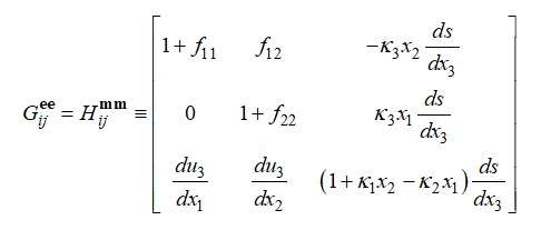
The deformation gradient can also be decomposed as

$F=RG=HR$

where R is the rigid rotation satisfying $m_i=R{e}_i$, and G and H are deformation gradient like tensors that describe the change in shape of the rod.  These tensors are most conveniently expressed as components in  $\left\{e_1,e_2,e_3\right\}$ and $\left\{m_1,m_2,m_3\right\}$, respectively $–$ we can represent this in diadic notation as $G=G_{ij}^{ee}{e}_i\otimes e_j$ or $H=H_{ij}^{mm}{m}_i\otimes m_j$.  The components can be expressed in matrix form as

 

 

 

Derivation: The deformation gradient is, by definition, the derivative of the position vector of material particles with respect to their position in the reference configuration, i.e.

$F={\displaystyle \frac{dy}{dx}={\displaystyle \frac{dr}{d{x}_3}\otimes e_3+{\displaystyle \frac{d{\eta }_i}{d{x}_j}{m}_i\otimes e_j+{\eta }_i(x_j){\displaystyle \frac{d{m}_i}{d{x}_3}\otimes e_3}}}}$

To reduce this to the expression given,

 

1. Note that

${\displaystyle \frac{dr}{d{x}_3}={\displaystyle \frac{dr}{ds}{\displaystyle \frac{ds}{d{x}_3}=m_3{\displaystyle \frac{ds}{d{x}_3}{\displaystyle \frac{d{m}_i}{d{x}_3}={\displaystyle \frac{d{m}_i}{ds}{\displaystyle \frac{ds}{d{x}_3}}}}}}}}$

 

2. Recall that

${\displaystyle \frac{d{m}_1}{ds}=-{\kappa }_2{m}_3+{\kappa }_3{m}_2{\displaystyle \frac{d{m}_2}{ds}={\kappa }_1{m}_3-{\kappa }_3{m}_1{\displaystyle \frac{d{m}_3}{ds}=-{\kappa }_1{m}_2+{\kappa }_2{m}_1}}}$

 

3. Substitute ${\eta }_{\alpha }=x_{\alpha }+f_{\alpha \beta }(x_3)x_{\beta },{\eta }_3=u_3(x_{\beta },x_3)$ and neglect the derivatives of f and $u_3$ with respect to $x_3$

 

The decomposition $F=RG$ follows trivially by substituting $m_i=R{e}_i$ into the dyadic representation of F and rearranging the result.  A similar approach gives $F=HR$.

 

 

 

10.2.6 Other strain measures

 

It is straightforward to compute additional strain measures from the deformation gradient.  Only a partial list will be given here.

 

1. The determinant of the deformation gradient follows as

$J=\det (F)=\det (G)=\det (H)=(1+f_{11})(1+f_{22})\left(1+{\kappa }_1{x}_2-{\kappa }_2{x}_1\right){\displaystyle \frac{ds}{d{x}_3}\approx {\displaystyle \frac{ds}{d{x}_3}}}$

 

2. The components of the left and right Cauchy-Green tensors can be computed from $B=F{F}^T=H{H}^T$ and $C=F^{T}F=G^{T}G$, where G and H were defined in 10.2.4.   C and B are most conveniently expressed as components in $\left\{e_1,e_2,e_3\right\}$ and $\left\{m_1,m_2,m_3\right\}$, respectively $–$ we can represent this in diadic notation as $C=C_{ij}^{ee}{e}_i\otimes e_j$ or $B=B_{ij}^{mm}{m}_i\otimes m_j$. For small distorsions, the result can be approximated by

 

 

3. The Lagrange strain is defined as $E=(C-I)/2$.  Its components follow trivially from the preceding formula.  Note that the matrix of components for E resembles the formula for the infinitesimal strain components in a straight bar subjected to axial stretching, bending and twist deformation.   However, if the bent rod does not lie in one plane, the twisting measure ${\kappa }_3$ includes contributions from both the rotation of the rod’s cross section about its axis, and also from the bending of the rod.

 

4. The rate of deformation tensor $D=\text{sym}(\dot{F}{F}^{-1})$ will also be required. It is simplest to calculate the velocity gradient $L=\dot{F}{F}^{-1}$ by differentiating the expression given for the velocity vector in the preceding section.

$\begin{array}{l}{\displaystyle \frac{dy}{dt}={\displaystyle \frac{dr}{dt}+{\dot{f}}_{\alpha \beta }{x}_{\beta }{m}_{\alpha }+x_{\alpha }\omega \times m_{\alpha }+{\dot{u}}_3{m}_3}}\\ \Rightarrow \dot{F}={\displaystyle \frac{d}{dt}\left({\displaystyle \frac{ds}{d{x}_3}{\displaystyle \frac{dr}{ds}}}\right)\otimes e_3+\left[{\dot{f}}_{\alpha \beta }{m}_{\alpha }+{\displaystyle \frac{\partial {\dot{u}}_3}{\partial x_{\beta }}{m}_3}\right]\otimes e_{\beta }+{\dot{f}}_{\alpha \beta }{x}_{\beta }{\displaystyle \frac{ds}{d{x}_3}{\displaystyle \frac{d{m}_{\alpha }}{ds}\otimes e_3}}}\\ +\left(\omega \times m_{\alpha }\right)\otimes e_{\alpha }+{\displaystyle \frac{ds}{d{x}_3}{\displaystyle \frac{d}{ds}\left(\omega \times m_{\alpha }\right)\otimes e_3+{\dot{u}}_3{\displaystyle \frac{ds}{d{x}_3}{\displaystyle \frac{d{m}_3}{ds}\otimes e_3}}}}\end{array}$

Substitute $dr/ds=m_3,d{m}_i/ds=\kappa \times m_i,d\omega /ds=\stackrel{\nabla }{\kappa }$, and note that

$\begin{array}{l}{F}^{-1}\approx {\displaystyle \frac{d{x}_3}{ds}(1+{\kappa }_2{x}_1-{\kappa }_1{x}_2)e_3\otimes m_3-{\displaystyle \frac{ds}{d{x}_3}{x}_1{\kappa }_3{e}_2\otimes m_3+{\displaystyle \frac{ds}{d{x}_3}{x}_2{\kappa }_3{e}_1\otimes m_3}}}\\ +({\delta }_{\alpha \beta }-f_{\alpha \beta })e_{\alpha }\otimes m_{\beta }-{\displaystyle \frac{d{u}_3}{d{x}_{\beta }}{e}_3\otimes m_{\beta }}\end{array}$

Evaluating $D=\text{sym}(\dot{F}{F}^{-1})$ then shows that the components of D in $\left\{m_1,m_2,m_3\right\}$ are

 

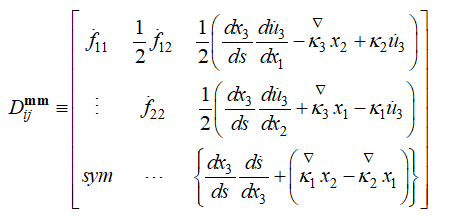
to within second order terms in curvature, $f_{ij}$ and $d{u}_3/d{x}_{\alpha }$.

 

 

 

10.2.7 Kinematics of rods that are bent and twisted in the unstressed state

 

It is straightforward to generalize the results in sections 10.2.3-10.2.5 to calculate strain measures for rods that are not straight in their initial configuration, as shown below.

 

In this case we must start by describing the geometry of the undeformed rod.  To this end

 

1. We denote the distance measured along the axis of the initial, unstressed, twisted rod by $\overline{s}$

 

2. At each point $\overline{s}$ on the initial rod, we introduce a set of three mutually perpendicular unit vectors $\{{\overline{m}}_1,{\overline{m}}_2,{\overline{m}}_3\}$, where ${\overline{m}}_3$ is chosen to be tangent to the axis of the undeformed rod; while ${\overline{m}}_1,{\overline{m}}_2$ are parallel to the principal moments of inertia of the cross-section.

 

3.  We also introduce an arbitrary Cartesian basis $\{e_1,e_2,e_3\}$ where the unit vectors denote three fixed directions in space.

 

4. The basis vectors $\{e_1,e_2,e_3\}$ and $\{{\overline{m}}_1,{\overline{m}}_2,{\overline{m}}_3\}$ together define a set of three Euler angles $\left(\overline{\varphi }(s),\overline{\theta }(s),\overline{\psi }(s)\right)$, which completely describe the shape of the undeformed rod.

 

5. We define a rotation tensor $\overline{R}$ satisfying ${\overline{m}}_i=\overline{R}{e}_i$ that characterizes the orientation of $\{{\overline{m}}_1,{\overline{m}}_2,{\overline{m}}_3\}$ with respect to $\{e_1,e_2,e_3\}$.  The components of $\overline{R}$ can be found using the formulas in Section 10.2.3.

 

6. We define three curvature components ${\overline{\kappa }}_i$ that characterize the bending and twisting of the initial rod, as follows

$\begin{array}{l}{\overline{\kappa }}_1=\sin (\overline{\psi }){\displaystyle \frac{d\overline{\theta }}{d\overline{s}}-\cos (\overline{\psi })\sin \overline{\theta }{\displaystyle \frac{d\overline{\varphi }}{d\overline{s}}}}\\ {\overline{\kappa }}_2=\cos (\overline{\psi }){\displaystyle \frac{d\overline{\theta }}{d\overline{s}}+\sin (\overline{\psi })\sin \overline{\theta }{\displaystyle \frac{d\overline{\varphi }}{d\overline{s}}}}\\ {\overline{\kappa }}_3={\displaystyle \frac{d\overline{\psi }}{d\overline{s}}+{\displaystyle \frac{d\overline{\varphi }}{d\overline{s}}\cos \overline{\theta }}}\end{array}$

 

 

The deformed shape of the rod is characterized exactly as described in Section 10.2.1, except that the axial distance $x_3$ is replaced by the arc-length $\overline{s}$ of the undeformed rod.

 

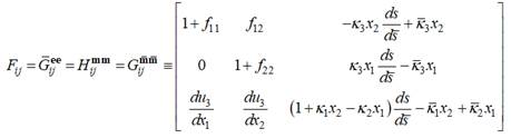
Assuming small distorsions, the deformation gradient can be expressed in dyadic notation as $F=F_{ij}{m}_i\otimes {\overline{m}}_j$, where the coefficients $F_{ij}$ are given below.  The deformation gradient can also be decomposed into two successive rotations and a small distorsion

$F=R\overline{G}{\overline{R}}^T=HR{\overline{R}}^T=R{\overline{R}}^{T}G$

where the rotation tensors $R$ and $\overline{R}$ satisfy ${\overline{m}}_i=\overline{R}{e}_i{m}_i=R{e}_i{m}_i=R{\overline{R}}^T{\overline{m}}_i$, and the tensors $\overline{G},H,G$ can be expressed in component form as   $\overline{G}={\overline{G}}_{ij}^{ee}{e}_i\otimes e_j,H_{ij}^{mm}{m}_i\otimes m_j,G_{ij}^{\overline{m}\overline{m}}{\overline{m}}_i\otimes {\overline{m}}_j$.  Their components are given by

 

 

The deformation gradient can be written down immediately, by mapping the initial rod onto a fictitious intermediate configuration in which the rod is straight, chosen as follows:

 

1. The straight rod has axis parallel to the $e_3$ direction

 

2. The point at arc-length $\overline{s}$ in the unstressed rod has coordinates $x=\overline{s}{e}_3$ in the intermediate configuration.

 

3. The principal axes of the cross section are parallel to $(e_1,e_2)$ in the intermediate configuration

 

4. The cross-section of the rod has the same shape in the intermediate configuration as in the undeformed configuration.

 

The deformed state can be reached in two steps (i) Deform the rod from the unstressed configuration to the intermediate configuration, with a deformation gradient $\overline{F}$.  The components of $\overline{F}$ can be calculated as the inverse of the deformation gradient that maps the intermediate straight rod onto the undeformed shape.  (ii) Deform the rod from the straight configuration to the deformed configuration, with a deformation gradient $\widehat{F}$.  The total deformation gradient follows as $F=\widehat{F}\overline{F}$. 

 

 

 

10.2.8 Representation of forces and moments in slender rods

 

The figure shows a generic cross-section of the rod, in the deformed configuration. To describe measures of internal and external force acting on the rod, we first define a basis $\{m_1,m_2,m_3\}$, with the unit vectors chosen using the scheme described in 10.2.2.  We then define the following vector components in this basis:

 

· The body force acting on the rod $b_i$.  For simplicity, we shall assume that the body force is uniform within the cross section (but $b_i$ may vary along the length of the rod).

 

· The tractions acting on the exterior surface of the rod $t_i$

 

· The Cauchy stress within the rod ${\sigma }_{ij}$.

 

 

External forces and moments acting on the rod are characterized by

 

1. The force per unit length acting on the rod, $p=p_i{m}_i$.  The force components can be calculated from the tractions and body force acting on the rod as $f_i(x_3)=A{b}_i+{\displaystyle \underset{C}{\int }{t}_{i}ds}$

 

2. The moment per unit length acting on the rod, $q=q_i{m}_i$.  The moment components can  be calculated from the tractions acting on the exterior surface of the rod as as

$q_1={\displaystyle \underset{C}{\int }{x}_2{t}_{3}ds}{q}_2=-{\displaystyle \underset{C}{\int }{x}_1{t}_{3}ds}{q}_3={\displaystyle \underset{C}{\int }(x_1{t}_2-x_2{t}_1)ds}$

 

3. The resultant force acting on each end of the rod.  Each force can be expressed as components as $P=P_i{m}_i$.  The components are related to the tractions acting on the end of the rod by $P_i={\displaystyle \underset{A}{\int }{t}_{i}dA}$, where the area integral is taken over the cross section at the appropriate end of the rod.

 

4. The resultant moment acting on each end of the rod.  Each moment can be expressed as components as $Q=Q_i{m}_i$.  The components are related to the tractions acting on the end of the rod by

$Q_1={\displaystyle \underset{A}{\int }{x}_2{t}_{3}dA{Q}_2}=-{\displaystyle \underset{A}{\int }{x}_1{t}_{3}dA}{Q}_3={\displaystyle \underset{A}{\int }(x_1{t}_2-x_2{t}_1)dA}$

 

 

Internal forces and moments in the rod are characterized by the following quantities:

 

1. The variation of internal shear stress in the cross section ${\sigma }_{\alpha 3}(x_{\beta },x_3)$

 

2. The average in-plane stress components

$S_{\alpha \beta }={\displaystyle \underset{A}{\int }{\sigma }_{\alpha \beta }dA}$

 

3. Three components of a vector bending moment, defined as

$M_1(x_3)={\displaystyle \underset{A}{\int }{\sigma }_{33}{x}_{2}dA}{M}_2(x_3)=-{\displaystyle \underset{A}{\int }{\sigma }_{33}{x}_{1}dA}{M}_3(x_3)={\displaystyle \underset{A}{\int }\left({\sigma }_{23}{x}_1-{\sigma }_{13}{x}_2\right)}dA$

 

4. The axial force on the cross-section $T_3(x_3)={\displaystyle \underset{A}{\int }{\sigma }_{33}dA}$

 

5. Two additional generalized forces $T_1(x_3),T_2(x_3)$, which represent the transverse shear forces acting on the rod’s cross section.  Unlike the axial force, however, these forces cannot be directly related to the deformation of the rod.  Instead, they are calculated from the bending moments, using the equilibrium equations listed in the next section.  

 

 

The forces $T_i$ and moments $M_i$ define components of a vector force and moment

 

1. $T=T_i{m}_i$ is the resultant force acting on an internal cross-section of the rod;

 

2. $M=M_i{m}_i$ is the resultant moment (about the centroid of the cross section) acting on the cross-section.

 

 

 

10.2.9 Equations of motion and boundary conditions

 

The internal forces and moments must satisfy the equations of motion

 ${\displaystyle \frac{\partial {\sigma }_{\alpha 3}}{\partial x_{\alpha }}-{\sigma }_{31}{\kappa }_2+{\sigma }_{32}{\kappa }_1=0}$       

${\displaystyle \frac{dT}{ds}+p=\rho Aa{\displaystyle \frac{dM}{ds}+m_3\times T+q=\rho {\rm H}\alpha +\omega \times \rho {\rm H}\omega }}$

Here, ${\sigma }_{\alpha 3}$, T and M are the internal forces and moments in the rod; $p,q$ are the external force and couple per unit length; $\rho$ is the mass density of the rod; A is its cross-sectional area, H is the area moment of inertia tensor defined in Sect 10.2.1, while $a,\omega ,\alpha$ are the acceleration, angular velocity and angular acceleration of the rod’s centerline, respectively. The two equations of motion for T and M clearly represent linear and angular moment balance for an infinitesimal segment of the rod.

 

The equations of motion for T and M are often expressed as components in the $\left\{m_1,m_2,m_3\right\}$ basis, as

$\begin{array}{l}{\displaystyle \frac{d{T}_1}{ds}-{\kappa }_3{T}_2+{\kappa }_2{T}_3+p_1=\rho A{a}_1}\\ {\displaystyle \frac{d{T}_2}{ds}+{\kappa }_3{T}_2-{\kappa }_1{T}_3+p_2=\rho A{a}_2}\\ {\displaystyle \frac{d{T}_3}{ds}+{\kappa }_1{T}_2-{\kappa }_2{T}_1+p_3=\rho A{a}_3}\end{array}$

$\begin{array}{l}{\displaystyle \frac{d{M}_1}{ds}-{\kappa }_3{M}_2+{\kappa }_2{M}_3-T_2+q_1=\rho I_1{\alpha }_1+\rho (I_3-I_2){\omega }_2{\omega }_3}\\ {\displaystyle \frac{d{M}_2}{ds}+{\kappa }_3{M}_1-{\kappa }_1{M}_3+T_1+q_2=\rho I_2{\alpha }_2-\rho (I_3-I_1){\omega }_1{\omega }_3}\\ {\displaystyle \frac{d{M}_3}{ds}-{\kappa }_2{M}_1+{\kappa }_1{M}_2+q_3=I_3{\alpha }_3+(I_2-I_1){\omega }_2{\omega }_1}\end{array}$

 

Note that:

 

1. If the system is in static equilibrium, the right hand sides of all the equations of motion are zero.

 

2. In addition, in many dynamic problems, the right hand sides of the angular momentum balance equations may be taken to be approximately zero, since the area moments of inertia are small.   For example, the rotational inertia may be ignored when modeling the vibration of a beam.  The rotational inertia terms can be important if the rod is rotating rapidly: examples include a spinning shaft, or a rotating propeller.

 

 

Boundary Conditions: The internal stresses, forces and moments must satisfy the following boundary conditions

 

1. $S_{\alpha \beta }={\displaystyle \underset{C}{\int }\left(x_{\beta }{t}_{\alpha }\right)d\xi }$

 

2. ${\sigma }_{3\alpha }{n}_{\alpha }=t_3$ on C

 

3. The ends of the rod may be subjected to a prescribed displacement.   Alternatively, the transverse or axial tractions may be prescribed on the ends of the bar: in this case the internal forces must satisfy $T=P$ for $s=L$ and $T=-P$ for s=0.

 

4. The ends of the rod may be subjected to a prescribed rotation.  Alternatively, if the ends are free to rotate, the internal moments must satisfy $M=Q$ for $s=L$ and $M=-Q$ for s=0.

 

 

Derivation: Measures of internal force and the equilibrium equations emerge naturally from the principle of virtual work, which states that the Cauchy stress distribution must satisfy

${\displaystyle \underset{V_0}{\int }J{\sigma }_{ij}\delta D_{ij}d{V}_0}+{\displaystyle \underset{V_0}{\int }\rho {\displaystyle \frac{d^2{y}_i}{d{t}^2}\delta v_{i}d{V}_0}}-{\displaystyle \underset{V_0}{\int }{b}_i\delta v_{i}d{V}_0}-{\displaystyle \underset{S_2}{\int }{t}_i\delta v_{i}dA}=0$

for all virtual velocity fields $\delta v_i$ and compatible stretch rates $\delta D_{ij}$.  The virtual velocity field and virtual stretch rates in the bar must have the same general form as the actual velocity and stretch rates, as outlined in Section 10.2.4 and 10.2.5.  The virtual velocity and stretch rate can therefore be characterized by $\delta {\dot{f}}_{\alpha \beta },\delta u_3(x_{\alpha })$ and compatible sets of $\delta v,\delta \omega ,\delta \dot{s},\delta {\stackrel{\nabla }{\kappa }}_i$.  This has two consequences:

 

· The virtual work principle can be expressed in terms of the generalized deformation measures and forces defined in the preceding sections as

$\begin{array}{l}{\displaystyle \underset{0}{\overset{L_0}{\int }}\left\{{\displaystyle \frac{ds}{d{x}_3}{S}_{\alpha \beta }\delta {\dot{f}}_{\alpha \beta }+{\displaystyle \underset{A}{\int }\left({\sigma }_{\alpha 3}{\displaystyle \frac{d\delta {\dot{u}}_3}{d{x}_{\alpha }}+({\sigma }_{31}{\kappa }_2-{\sigma }_{32}{\kappa }_1)\delta {\dot{u}}_3-b_3\delta {\dot{u}}_3}\right)dA}}\right\}d{x}_3}\\ +{\displaystyle \underset{0}{\overset{L_0}{\int }}\left\{{\displaystyle \frac{d\delta \dot{s}}{d{x}_3}{T}_3+\delta {\stackrel{\nabla }{\kappa }}_i{M}_i{\displaystyle \frac{ds}{d{x}_3}}}\right\}d{x}_3}+{\displaystyle \underset{0}{\overset{L}{\int }}\rho A{a}_i\delta v_i}ds\\ +{\displaystyle \underset{0}{\overset{L}{\int }}\rho I_1\left({\alpha }_1+{\omega }_2{\omega }_3\right)\delta {\omega }_1}ds+{\displaystyle \underset{0}{\overset{L}{\int }}\rho I_2\left({\alpha }_2-{\omega }_1{\omega }_3\right)\delta {\omega }_2}ds+{\displaystyle \underset{0}{\overset{L}{\int }}\rho \left(I_3{\alpha }_3+(I_1-I_2){\omega }_1{\omega }_2\right)\delta {\omega }_3}ds\\ -{\displaystyle \underset{0}{\overset{L}{\int }}\left({\displaystyle \underset{C}{\int }\left(x_{\beta }{t}_{\alpha }\delta {\dot{f}}_{\alpha \beta }+t_3\delta u_3\right)d\xi }\right)}ds-{\displaystyle \underset{0}{\overset{L}{\int }}\left(p_i\delta v_i+q_i\delta {\omega }_i\right)}ds\\ -{\left[P_i\delta v_i+Q_i\delta {\omega }_i\right]}_{x_3=0}-{\left[P_i\delta v_i+Q_i\delta {\omega }_i\right]}_{x_3=L_0}=0\end{array}$

 

· If the virtual work equation is satisfied for all $\delta {\dot{f}}_{\alpha \beta },\delta u_3(x_{\alpha })$ and compatible sets of $\delta v,\delta \omega ,\delta \dot{s},\delta {\stackrel{\nabla }{\kappa }}_i$, then the internal forces and moments must satisfy the equilibrium equations and boundary conditions listed above.

 

 

It is straightforward to derive the first result.  The Jacobian is approximated as $J\approx ds/d{x}_3$; the components of  $\delta D_{ij}$ follow from the formulas given in Section 10.2.6, and the velocity field is approximated using the formula in 10.2.5.  Substituting the definitions given in Section 10.2.7 for generalized internal and external forces immediately gives the required result.  The algebra involved is lengthy and tedious and is left as an exercise.

 

The equilibrium equations and boundary conditions are obtained by substituting various choices of $\delta {\dot{f}}_{\alpha \beta },\delta u_3(x_{\alpha })$ and compatible sets of $\delta v,\delta \omega ,\delta \dot{\psi },\delta \dot{s},\delta {\stackrel{\nabla }{\kappa }}_i$ into the virtual work equation.

 

1. Choosing $\delta u_3(x_{\alpha })=\delta v=\delta \dot{\psi }=0$ reduces the virtual work equation to

${\displaystyle \underset{0}{\overset{L_0}{\int }}\left\{{\displaystyle \underset{A}{\int }{\sigma }_{\alpha \beta }\delta {\dot{f}}_{\alpha \beta }}dA\right\}d{x}_3}-{\displaystyle \underset{0}{\overset{L}{\int }}\left({\displaystyle \underset{C}{\int }\left(x_{\beta }{t}_{\alpha }\delta {\dot{f}}_{\alpha \beta }\right)d\xi }\right)}ds$

The condition $S_{\alpha \beta }={\displaystyle \underset{C}{\int }\left(x_{\beta }{t}_{\alpha }\right)d\xi }$ follows immediately. 

 

2. Choosing $\delta f_{\alpha \beta }=\delta v=\delta \dot{\psi }=0$ reduces the virtual work equation to

${\displaystyle \underset{0}{\overset{L_0}{\int }}\left\{{\displaystyle \underset{A}{\int }\left({\sigma }_{\alpha 3}{\displaystyle \frac{d\delta {\dot{u}}_3}{d{x}_{\alpha }}+({\sigma }_{31}{\kappa }_2-{\sigma }_{32}{\kappa }_1)\delta {\dot{u}}_3-b_3\delta {\dot{u}}_3}\right)dA}\right\}d{x}_3}-{\displaystyle \underset{0}{\overset{L_0}{\int }}\left({\displaystyle \underset{C}{\int }\left(t_3\delta {\dot{u}}_3\right)d\xi }\right)}{\displaystyle \frac{ds}{d{x}_3}d{x}_3}$

Recall that (by definition) $\delta {\dot{u}}_3$ must be chosen to satisfy

${\displaystyle \underset{A}{\int }\delta {\dot{u}}_{3}dA}=0$

Since the body force is uniform, the term involving $b_3$ is zero.  The first integral can then be integrated by parts as follows

${\displaystyle \underset{A}{\int }{\sigma }_{\alpha 3}{\displaystyle \frac{\partial \delta u_3}{\partial x_{\alpha }}dA}}={\displaystyle \underset{A}{\int }\left({\displaystyle \frac{\partial }{\partial x_{\alpha }}\left({\sigma }_{\alpha 3}\delta u_3\right)-{\displaystyle \frac{\partial {\sigma }_{\alpha 3}}{\partial x_{\alpha }}\delta u_3}}\right)dA}={\displaystyle \underset{C}{\int }{\sigma }_{\alpha 3}\delta u_3{n}_{\alpha }}-{\displaystyle \underset{A}{\int }\delta u_3{\displaystyle \frac{\partial {\sigma }_{\alpha 3}}{\partial x_{\alpha }}dA}}$

Choosing $\delta u_3$ to vanish on the boundary or the interior yields the equilibrium equation

 $\partial {\sigma }_{\alpha 3}/\partial x_{\alpha }-{\sigma }_{31}{\kappa }_2+{\sigma }_{32}{\kappa }_1=0$

choosing any other $\delta u_3$ gives the boundary condition ${\sigma }_{3\alpha }{n}_{\alpha }=t_3$.

 

3. Choosing $\delta u_3(x_{\alpha })=f_{\alpha \beta }=\delta \dot{r}=0$, using $\delta {\stackrel{\nabla }{\kappa }}_1=\delta \dot{\psi }{\kappa }_2\delta {\stackrel{\nabla }{\kappa }}_2=-\delta \dot{\psi }{\kappa }_1\delta {\stackrel{\nabla }{\kappa }}_3=d\delta \dot{\psi }/ds$ as well as $\delta {\omega }_3=\delta \dot{\psi }$ yields

$\begin{array}{l}{\displaystyle \underset{0}{\overset{L_0}{\int }}\left\{\left(+{\kappa }_2{M}_1-{\kappa }_1{M}_2\right)\delta \dot{\psi }+{\displaystyle \frac{d\delta \dot{\psi }}{ds}{M}_3}\right\}d{x}_3+{\displaystyle \underset{0}{\overset{L}{\int }}\rho \left(I_3{\alpha }_3+(I_1-I_2){\omega }_1{\omega }_2\right)\delta \dot{\psi }}ds}\\ -{\displaystyle \underset{0}{\overset{L}{\int }}\left(q_3\delta \dot{\psi }\right)}ds-{\left[Q_3\delta \dot{\psi }\right]}_{x_3=0}-{\left[Q_3\delta \dot{\psi }\right]}_{x_3=L_0}=0\\ \Rightarrow {\displaystyle \underset{0}{\overset{L_0}{\int }}\left\{\left(-{\displaystyle \frac{d{M}_3}{ds}+{\kappa }_2{M}_1-{\kappa }_1{M}_2-q_3-\rho \left(I_3{\alpha }_3+(I_1-I_2){\omega }_1{\omega }_2\right)}\right)\delta \dot{\psi }\right\}d{x}_3}\\ +{\left[(M_3-Q_3)\delta \dot{\psi }\right]}_{x_3=L_0}-{\left[(M_3+Q_3)\delta \dot{\psi }\right]}_{x_3=0}=0\end{array}$

where we have integrated by parts to obtain the second line.   Choosing $\delta \dot{\psi }$ to vanish on the ends of the rod yields the equation of motion $d{M}_3/ds-{\kappa }_2{M}_1+{\kappa }_1{M}_2+q_3=\rho \left(I_3{\alpha }_3+(I_1-I_2){\omega }_1{\omega }_2\right)$. Any other choice of  $\delta \dot{\psi }$ yields the boundary conditions $M_3=\pm Q_3$ on the ends of the rod.

 

4. Choosing $\delta u_3(x_{\alpha })=f_{\alpha \beta }=\delta \dot{\psi }=0$ and substituting $\delta {\omega }_1=-\delta {\dot{\tau }}_2$, $\delta {\omega }_2=\delta {\dot{\tau }}_1$, where $\delta {\dot{\tau }}_{\alpha }$ are the components of a virtual rate of change of the tangent vector $t$ reduces the virtual work equation to

$\begin{array}{l}{\displaystyle \underset{0}{\overset{L_0}{\int }}\left\{{\displaystyle \frac{d\delta \dot{s}}{d{x}_3}{T}_3+\delta {\stackrel{\nabla }{\kappa }}_i{M}_i{\displaystyle \frac{ds}{d{x}_3}}}\right\}d{x}_3}-{\displaystyle \underset{0}{\overset{L}{\int }}\left(p_i\delta v_i-q_{2}d{\dot{\tau }}_1+q_1\delta {\dot{\tau }}_2\right)}ds\\ +{\displaystyle \underset{0}{\overset{L}{\int }}\rho A{a}_i\delta v_i}ds+{\displaystyle \underset{0}{\overset{L}{\int }}\rho I_1\left({\alpha }_1+{\omega }_2{\omega }_3\right)\delta {\dot{\tau }}_2}ds-{\displaystyle \underset{0}{\overset{L}{\int }}\rho I_2\left({\alpha }_2-{\omega }_1{\omega }_3\right)\delta {\dot{\tau }}_1}ds\\ -{\left[P_i\delta v_i-Q_2\delta {\dot{\tau }}_1+Q_1\delta {\dot{\tau }}_2\right]}_{x_3=0}-{\left[P_i\delta v_i-Q_2\delta {\dot{\tau }}_1+Q_1\delta {\dot{\tau }}_2\right]}_{x_3=L_0}=0\end{array}$

To proceed, it is necessary to express $\delta {\dot{\kappa }}_i,\delta {\dot{\tau }}_i$ and $\delta \dot{s}$ in terms of the virtual velocity components $\delta v_i$. The algebra and the resulting equilibrium equations are greatly simplified if the tangent vector $t$ is regarded as an independent kinematic variable.   The relationship between t and $dr/ds$ must be enforced by a vector valued Lagrange multiplier $T^{\prime }=T_1{m}_1+T_2{m}_2$, which must satisfy

${\displaystyle \underset{0}{\overset{L}{\int }}\left({\displaystyle \frac{dr}{ds}-t}\right)\cdot \delta {\dot{T}}^{\prime }ds}+{\displaystyle \underset{0}{\overset{L}{\int }}\left({\displaystyle \frac{d\delta v}{ds}-\delta \dot{t}}\right)\cdot T^{\prime }ds}=0$

for all variations $\delta \dot{t},\delta \dot{r},\delta {\dot{T}}^{\prime }$. The second integral can be expressed in component form as

${\displaystyle \underset{0}{\overset{L}{\int }}\left({\displaystyle \frac{d\delta v_{\alpha }}{ds}{T}_{\alpha }+\left(-\delta v_2{\kappa }_3+\delta v_3{\kappa }_2\right)T_1+\left(\delta v_1{\kappa }_3-\delta v_3{\kappa }_1\right)T_2-\delta {\dot{\tau }}_{\alpha }{T}_{\alpha }}\right)}ds=0$

This equation can simply be added to the virtual work equation to ensure that $\delta {\dot{\tau }}_{\alpha }$ and $\delta v_i$ are consistent.   Finally, recall that the curvature rates and stretch rate are related to $\delta v_i$ $\delta {\dot{\tau }}_{\alpha }$ by

$\begin{array}{l}{\displaystyle \frac{d\delta \dot{s}}{d{x}_3}={\displaystyle \frac{ds}{d{x}_3}\left({\displaystyle \frac{d\delta v_3}{ds}-\delta v_1{\kappa }_2+\delta v_2{\kappa }_1}\right)}}\\ \delta \stackrel{\nabla }{{\kappa }_1}=-{\displaystyle \frac{d\delta {\dot{\tau }}_2}{ds}-\delta {\dot{\tau }}_1{\kappa }_3\delta \stackrel{\nabla }{{\kappa }_2}={\displaystyle \frac{d\delta {\dot{\tau }}_1}{ds}-\delta {\dot{\tau }}_2{\kappa }_3\delta \stackrel{\nabla }{{\kappa }_3}=\delta {\dot{\tau }}_1{\kappa }_1+\delta {\dot{\tau }}_2{\kappa }_2}}\end{array}$

Substituting these results into the augmented virtual work equation gives

$\begin{array}{l}{\displaystyle \underset{0}{\overset{L}{\int }}\left(\left({\displaystyle \frac{d\delta v_{\alpha }}{ds}{T}_{\alpha }+\delta v_1{\kappa }_3{T}_2-\delta v_2{\kappa }_3{T}_1+\delta v_3(-{\kappa }_1{T}_2+{\kappa }_2{T}_1)}\right)-\delta {\dot{\tau }}_{\alpha }{T}_{\alpha }\right)}ds\\ +{\displaystyle \underset{0}{\overset{L}{\int }}\left\{\left({\displaystyle \frac{d\delta v_3}{ds}+\left(-\delta v_1{\kappa }_2+\delta v_2{\kappa }_1\right)}\right)T_3\right\}}ds\\ +{\displaystyle \underset{0}{\overset{L}{\int }}\rho A{a}_i\delta v_i}ds+{\displaystyle \underset{0}{\overset{L}{\int }}\rho I_1\left({\alpha }_1+{\omega }_2{\omega }_3\right)\delta {\dot{\tau }}_2}ds-{\displaystyle \underset{0}{\overset{L}{\int }}\rho I_2\left({\alpha }_2-{\omega }_1{\omega }_3\right)\delta {\dot{\tau }}_1}ds\\ +{\displaystyle \underset{0}{\overset{{}_L}{\int }}\left\{\left(-{\displaystyle \frac{d\delta {\dot{\tau }}_2}{ds}-{\kappa }_3\delta {\dot{\tau }}_1}\right)M_1+\left({\displaystyle \frac{d\delta {\dot{\tau }}_1}{ds}-{\kappa }_3\delta {\dot{\tau }}_2}\right)M_2+\left({\kappa }_1\delta {\dot{\tau }}_1+{\kappa }_2\delta {\dot{\tau }}_2\right)M_3\right\}}ds\\ -{\displaystyle \underset{0}{\overset{L}{\int }}\left(p_i\delta v_i+q_2\delta {\dot{\tau }}_1-q_1\delta {\dot{\tau }}_2\right)}ds\\ -{\left[P_i\delta v_i+Q_2\delta {\dot{\tau }}_1-Q_1\delta {\dot{\tau }}_2\right]}_{x_3=0}-{\left[P_i\delta v_i+Q_2\delta {\dot{\tau }}_1-Q_1\delta {\dot{\tau }}_2\right]}_{x_3=L_0}=0\end{array}$

This equation must be satisfied for all admissible $\delta v_i,\delta {\dot{\tau }}_{\alpha }$. Considering each component in turn, and integrating by parts appropriately and using $I_3=I_1+I_2$ gives the last five equations of motion, as well as the boundary conditions $T=\pm PM=\pm Q$ on s=0 and s=L. 

 

 

 

10.2.10 Constitutive equations relating forces to deformation measures in elastic rods

 

Constitutive equations must relate the deformation measures defined in Section 10.2.3 to the forces defined in 10.2.8.  In this section we list the relationships between these quantities for an isotropic, elastic rod that is subjected to small distorsions.  For simplicity, the sides of the rod are assumed to be traction free.

 

The results depend on the geometry of the rod’s cross-section, which is characterized as follows. 

 

1. Introduce a Cartesian coordinate system $(x_1,x_2,x_3)$ as shown in the figure. The coordinates have origin at the centroid of the cross-section, with basis vectors $e_1,e_2$ parallel to the principal axes of inertia for the cross-section, and $e_3$ parallel to the rod’s axis.

 

2. We denote the cross-sectional area of the rod by A, and the curve bounding the cross-section by C, and let $I_i$ denote the three principal moments of area of the cross-section (see Sect 10.2.1).

 

3. We introduce a warping function $w(x_1,x_2)$ to describe the out-of-plane displacement component $u_3$ in the cross-section of the rod.  The warping function is related to the out-of-plane displacement $u_3$ by

$u_3(x_1,x_2,x_3)=\left({\kappa }_3(x_3)-{\overline{\kappa }}_3(x_3)\right)w(x_1,x_2)$

The warping function depends only on the geometry of the cross-section, and satisfies the following governing equations and boundary conditions

$\begin{array}{l}{\displaystyle \frac{{\partial }^{2}w}{\partial x_1^2}+{\displaystyle \frac{{\partial }^{2}w}{\partial x_2^2}-{\displaystyle \frac{\partial w}{\partial x_1}{\kappa }_2+{\displaystyle \frac{\partial w}{\partial x_2}{\kappa }_1=0\text{in A}}}}}\\ {\displaystyle \frac{\partial w}{\partial x_{\alpha }}{n}_{\alpha }=x_2{n}_1-x_1{n}_2=x_{\alpha }{\displaystyle \frac{\partial x_{\alpha }}{\partial s}\text{on C}}}\end{array}$

You can easily show that this choice of $u_3$ will automatically satisfy the shear stress equilibrium equation $\partial {\sigma }_{\alpha 3}/\partial x_{\alpha }-{\sigma }_{31}{\kappa }_2+{\sigma }_{32}{\kappa }_1=0$ as well as the boundary condition ${\sigma }_{3\alpha }{n}_{\alpha }=0$ on C.

 

4. Finally we define a modified polar moment of inertia for the cross section as

$J_3=I_3-{\displaystyle \underset{A}{\int }\left(x_2{\displaystyle \frac{\partial w}{\partial x_1}-x_1{\displaystyle \frac{\partial w}{\partial x_2}}}\right)}dA$

 

 

Calculating the warping function is a nuisance, because it requires the solution to a PDE.  In desperation, you can take w=0 $–$ this will overestimate the torsional stiffness of the rod, but in many practical applications the error is not significant.   For a better approximation, warping functions can be estimated by neglecting the terms involving ${\kappa }_{\beta }\partial w/\partial x_{\alpha }$ in the governing equation.  A few such approximate warping functions and modified polar moments of area are listed in the table below. 

 

The force-deformation relations for the rod are

$\begin{array}{l}{T}_3={\displaystyle \frac{EA}{2}\left({\left({\displaystyle \frac{ds}{d\overline{s}}}\right)}^2-1\right)\approx EA\left({\displaystyle \frac{ds}{d\overline{s}}-1}\right)}\\ M_{\alpha }=E{I}_{\alpha }({\kappa }_{\alpha }-{\overline{\kappa }}_{\alpha })M_3=\mu J_3({\kappa }_3-{\overline{\kappa }}_3)\\ {\sigma }_{13}=\mu ({\kappa }_3-{\overline{\kappa }}_3)\left({\displaystyle \frac{\partial w}{\partial x_1}-x_2}\right){\sigma }_{23}=\mu ({\kappa }_3-{\overline{\kappa }}_3)\left({\displaystyle \frac{\partial w}{\partial x_2}+x_1}\right)\\ f_{11}=f_{22}=-{\displaystyle \frac{\nu }{2}\left\{{\left({\displaystyle \frac{ds}{d\overline{s}}}\right)}^2-1\right\}{f}_{12}=0}\end{array}$

The two shear force components $T_{\alpha }$ cannot be related to the deformation $–$ they are Lagrange multipliers that enforce the condition that the rod does not experience transverse shear, as discussed in the preceding section.

 

Derivation: These results can be derived as follows:

 

1. The elastic constitutive equations for materials subjected to small distorsions, but arbitrary rotations, are listed in Section 3.3.   They have the form

${\Sigma }_{ij}={\displaystyle \frac{E}{\left(1+\nu \right)}\left\{E_{ij}+{\displaystyle \frac{\nu }{1-2\nu }(E_{kk}){\delta }_{ij}}\right\}}$

where ${\Sigma }_{ij}$ are the components of the material stress tensor, and $E_{ij}$ are the components of the Lagrange strain tensor. The components of $E_{ij}^{ee}=(F_{ki}^{ee}{F}_{kj}^{ee}-{\delta }_{ij})/2$ in the basis $\{e_1,e_2,e_3\}$ can be found using the formulas for $F$ given in Section 10.2.7, and when substituted into the constitutive laws give expressions for the components of material stress ${\Sigma }_{ij}^{ee}$ in terms of the deformation measures $f_{\alpha \beta }$, $u_3$, ${\kappa }_i$ and $ds/d\overline{s}$.

 

2. The Cauchy stress is related to the material stress by $\sigma =F\Sigma F^T/J$.  For small distorsions, but arbitrary rotations, we may approximate this by $\sigma \approx R\Sigma R^T={\Sigma }_{ij}^{ee}R{e}_i\otimes R^T{e}_j={\Sigma }_{ij}^{ee}{m}_i\otimes m_j$, so the components of the material stress tensor in $\{e_1,e_2,e_3\}$ can be used as an approximation to the components of the Cauchy stress tensor in $\{m_1,m_2,m_3\}$.  

 

3. Since we have assumed that the tractions on the sides of the rod vanish, the in-plane stress components must satisfy ${\displaystyle \underset{A}{\int }{\sigma }_{\alpha \beta }dA}=0$.  Substituting the formulas for stresses from (2) and noting that ${\displaystyle \underset{A}{\int }{x}_{\alpha }}dA=0$  (because the origin for the coordinate system coincides with the centroid of the cross section) shows that $f_{11}=f_{22}=-\nu \left({(ds/d\overline{s})}^2-1\right)/2$, $f_{12}=0$, and

${\sigma }_{33}={\displaystyle \frac{E}{2}\left({\left({\displaystyle \frac{ds}{d\overline{s}}}\right)}^2-1+2({\kappa }_1-{\overline{\kappa }}_1)x_2-2({\kappa }_2-{\overline{\kappa }}_2)x_1\right)}$

 

4. Substituting the formula for ${\sigma }_{33}$ into the definitions of $T_3$, $M_1,M_2$ given in Section 10.2.8 and noting that ${\displaystyle \underset{A}{\int }{x}_1{x}_2}dA=0$ (because the basis vectors coincide with the principal axes of inertia) yields

$T_3={\displaystyle \frac{EA}{2}\left({\left({\displaystyle \frac{ds}{d\overline{s}}}\right)}^2-1\right)\approx EA\left({\displaystyle \frac{ds}{d\overline{s}}-1}\right)M_{\alpha }=E{I}_{\alpha }({\kappa }_{\alpha }-{\overline{\kappa }}_{\alpha })}$

 

5. Recall that the shear stress components ${\sigma }_{\alpha 3}$ must satisfy the equilibrium equation and boundary condition

${\displaystyle \frac{\partial {\sigma }_{\alpha 3}}{\partial x_{\alpha }}-{\sigma }_{31}{\kappa }_2+{\sigma }_{32}{\kappa }_1=0\text{in A}{\sigma }_{\alpha \beta }{n}_{\alpha }=0\text{on C}}$

Substituting the shear stress components from step (2) into this equilibrium equation and setting $u_3={\kappa }_{3}w$ gives the governing equation for w

$\begin{array}{l}{\displaystyle \frac{{\partial }^{2}w}{\partial x_1^2}+{\displaystyle \frac{{\partial }^{2}w}{\partial x_2^2}-{\displaystyle \frac{\partial w}{\partial x_1}{\kappa }_2+{\displaystyle \frac{\partial w}{\partial x_2}{\kappa }_1=0\text{in A}}}}}\\ {\displaystyle \frac{\partial w}{\partial x_{\alpha }}{n}_{\alpha }=x_2{n}_1-x_1{n}_2=x_{\alpha }{\displaystyle \frac{\partial x_{\alpha }}{\partial s}\text{on C}}}\end{array}$

 

6. The shear stresses now follow as

${\sigma }_{13}=\mu ({\kappa }_3-{\overline{\kappa }}_3)\left({\displaystyle \frac{\partial w}{\partial x_1}-x_2}\right){\sigma }_{23}=\mu ({\kappa }_3-{\overline{\kappa }}_3)\left({\displaystyle \frac{\partial w}{\partial x_2}+x_1}\right)$

Substituting these results into the equation defining $M_3$ in Section 10.2.6 gives the last equation

$M_3=\mu J_3({\kappa }_3-{\overline{\kappa }}_3)$

 

 

 

10.2.11 Strain energy of an elastic rod

 

The total strain energy of an elastic rod can be computed from its curvatures as

$\Phi ={\displaystyle \frac{1}{2}{\displaystyle \underset{0}{\overset{L}{\int }}\left\{EA{\left({\displaystyle \frac{ds}{d\overline{s}}-1}\right)}^2+E{I}_1{({\kappa }_1-{\overline{\kappa }}_1)}^2+E{I}_2{({\kappa }_2-{\overline{\kappa }}_2)}^2+\mu J_3{({\kappa }_3-{\overline{\kappa }}_3)}^2\right\}ds}}$

 

Derivation:  The derivation is similar to the procedure used to compute elastic moment-curvature relations.

1. The strain energy density in the rod can be computed from the Lagrange strain $E_{ij}$ and the Material Stress ${\Sigma }_{ij}$ as $U={\Sigma }_{ij}{E}_{ij}/2$.  The material stress can be related to the Lagrange strain using the formulas in Section 10.2.10, while the Lagrange strain can be expressed in terms of of the deformation measures $f_{\alpha \beta }$, $u_3$, ${\kappa }_i$ and $ds/d\overline{s}$ using the formulas for the deformation gradient listed in Sections 10.2.7.

 

2. The results can be simplified by recalling that $f_{11}=f_{22}=-\nu \left({(ds/d\overline{s})}^2-1\right)/2$, $f_{12}=0$, which shows that the strain energy density can be approximated as

$\begin{array}{l}U={\displaystyle \frac{E}{2}{\left(\left({\displaystyle \frac{ds}{d\overline{s}}-1}\right)+({\kappa }_1-{\overline{\kappa }}_1)x_2-({\kappa }_2-{\overline{\kappa }}_2)x_1\right)}^2}\\ +{\displaystyle \frac{\mu }{2}{\left({\kappa }_3-{\overline{\kappa }}_3\right)}^2\left\{{\left({\displaystyle \frac{\partial w}{\partial x_1}-x_2}\right)}^2+{\left({\displaystyle \frac{\partial w}{\partial x_2}+x_1}\right)}^2\right\}}\end{array}$

where w is the warping function defined in Section 10.2.9. The two terms in this expression represent the strain energy density due to stretching and bending the rod, and twisting the rod, respectively.

 

3. The total strain energy follows by integrating U over the volume of the rod.  Using the measures of cross-sectional geometry listed in Section 10.2.1, it is straightforward to show that

$\begin{array}{l}{\displaystyle \underset{V}{\int }{\displaystyle \frac{E}{2}{\left(\left({\displaystyle \frac{ds}{d\overline{s}}-1}\right)+({\kappa }_1-{\overline{\kappa }}_1)x_2-({\kappa }_2-{\overline{\kappa }}_2)x_1\right)}^2}}dV=\\ {\displaystyle \frac{E}{2}{\displaystyle \underset{0}{\overset{L}{\int }}\left\{A{\left({\displaystyle \frac{ds}{d\overline{s}}-1}\right)}^2+I_1{({\kappa }_1-{\overline{\kappa }}_1)}^2+I_2{({\kappa }_2-{\overline{\kappa }}_2)}^2\right\}ds}}\end{array}$

 

4. Some additional algebra is required to calculate the energy associated with twisting the rod. Begin by noting that

${\displaystyle \underset{A}{\int }\left\{{\left({\displaystyle \frac{\partial w}{\partial x_1}-x_2}\right)}^2+{\left({\displaystyle \frac{\partial w}{\partial x_2}+x_1}\right)}^2\right\}}dA=J+{\displaystyle \underset{A}{\int }\left({\displaystyle \frac{\partial w}{\partial x_{\alpha }}{\displaystyle \frac{\partial w}{\partial x_{\alpha }}-x_2{\displaystyle \frac{\partial w}{\partial x_1}+x_1{\displaystyle \frac{\partial w}{\partial x_2}}}}}\right)dA}$

We need to show that the integral on the right hand side of this expression is zero.

 

5. To this end, note that

${\displaystyle \underset{A}{\int }{\displaystyle \frac{\partial w}{\partial x_{\alpha }}}}{\displaystyle \frac{\partial w}{\partial x_{\alpha }}dA={\displaystyle \underset{A}{\int }{\displaystyle \frac{\partial }{\partial x_{\alpha }}\left(w{\displaystyle \frac{\partial w}{\partial x_{\alpha }}}\right)}}dA={\displaystyle \underset{C}{\int }w{\displaystyle \frac{\partial w}{\partial x_{\alpha }}{n}_{\alpha }ds}}={\displaystyle \underset{C}{\int }w\left(x_2{n}_1-x_1{n}_2\right)ds}}$

where we have recalled that the warping function w satisfies ${\partial }^{2}w/\partial x_{\alpha }\partial x_{\alpha }=0$ in A as well as $\left(\partial w/\partial x_{\alpha }\right)n_{\alpha }=x_2{n}_1-x_1{n}_2$ on C, and have used the divergence theorem.

 

6. Secondly, note that

$\begin{array}{l}{\displaystyle \underset{A}{\int }\left(-x_2{\displaystyle \frac{\partial w}{\partial x_1}+x_1{\displaystyle \frac{\partial w}{\partial x_2}}}\right)dA}={\displaystyle \underset{A}{\int }\left({\displaystyle \frac{\partial }{\partial x_1}\left(-x_{2}w\right)+{\displaystyle \frac{\partial }{\partial x_2}\left(w{x}_1\right)}}\right)dA}\\ ={\displaystyle \underset{C}{\int }\left(\left(-x_{2}w\right)n_1+\left(w{x}_1\right)n_2\right)dA}\end{array}$

The sum of (5) and (6) is zero.  Using this result and (4) gives the expression for the strain energy of the rod.