10.4 Exact solutions to simple problems involving elastic rods

 

This section lists solutions to various boundary and initial value problems involving deformable rods, to illustrate representative applications of the equations derived in Sections 10.2.2 and 10.2.3.   Specifically, we derive solutions for:

 

1. The natural frequencies and mode shapes for an initially straight vibrating beam;

 

2. The buckling load for a vertical rod subjected to gravitational loading;

 

3. The full post-buckled shape for a straight rod compressed by axial loads on its ends;

 

4. Internal forces and moments in an initially straight rod that is bent and twisted into a helix;

 

5. Internal forces, moments, and the deflected shape of a helical spring.

 

 

 

10.4.1 Free vibration of a straight beam without axial force

 

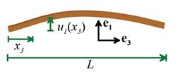The figure illustrates the problem to be solved: an initially straight beam, with axis parallel to the $e_3$ direction and principal axes of inertia parallel to $e_1,e_2$ is free of external force.  The beam has Young’s modulus $E$ and mass density $\rho$, and its cross-section has area A and principal moments of area $I_1,I_2,I_3$.  Its ends may be constrained in various ways, as described in more detail below.  We wish to calculate the natural frequencies and mode shapes of vibration for the beam, and to use these results to write down the displacement $u_1(x_3,t)$ for a beam that is caused to vibrate with initial conditions $u_1=u^0(x_3)$, $d{u}_1/dt=v^0(x_3)$ at time t=0.

 

Mode shapes and natural frequencies: The physical significance of the mode shapes and natural frequencies of a vibrating beam can be visualized as follows:

 

1. Suppose that the beam is made to vibrate by bending it into some (fixed) deformed shape $u_1=u^0(x_3)$; and then suddenly releasing it.   In general, the resulting motion of the beam will be very complicated, and may not even appear to be periodic.

 

2. However, there exists a set of special initial deflections $u^0=U_n(k_n{x}_3)$, which cause every point on the beam to experience simple harmonic motion at some (angular) frequency ${\omega }_n$, so that the deflected shape has the form $u_1(x,t)=U_n(k_n{x}_3)\cos ({\omega }_{n}t)$.

 

3. The special frequencies ${\omega }_n$ are called the natural frequencies of the beam, and the special initial deflections $U_n(k_n{x}_3)$ are called the mode shapes.   Each mode shape has a wave number $k_n$, which characterizes the wavelength of the harmonic vibrations, and is related to the natural frequency by

${\omega }_n=k_n^2\sqrt{{\displaystyle \frac{E{I}_2}{\rho A}}}$

 

4. The mode shapes $U_n$ have a very useful property (which is proved in Section 5.9.1):

${\displaystyle \underset{0}{\overset{L}{\int }}{U}_i(k_i{x}_3)}{U}_j(k_j{x}_3)=0i\ne j$

 

 

The mode shapes, wave numbers and corresponding natural frequencies depend on the way the beam is supported at its ends.  A few representative results are listed below

 

 

Beam with  free ends:

 

The wave numbers for each mode are given by the roots of the equation

 $\cos (k_{n}L)\cosh \left(k_{n}L\right)-1=0$

The mode shapes are

$U_n=A_n\left(\sinh (k_n{x}_3)+\sin (k_n{x}_3)+{\displaystyle \frac{\cosh (k_{n}L)-\cos (k_{n}L)}{\sinh (k_{n}L)+\sin (k_{n}L)}\left[\cosh (k_n{x}_3)+\cos (k_n{x}_3)\right]}\right)$

where $A_n$ are arbitrary constants.

 

 

Beam with pinned ends:

 

The wave numbers for each mode are $k_n=n\pi /L$

The mode shapes are $U_n=A_n\sin (k_n{x}_3)$, where $A_n$ are arbitrary constants.

 

 

Cantilever beam (clamped at $x_3=0$, free at  $x_3=L$ ):

 

The wave numbers for each mode are given by the roots of the equation

$\cos (k_{n}L)\cosh \left(k_{n}L\right)+1=0$

The mode shapes are

$U_n=A_n\left(\sinh (k_n{x}_3)-\sin (k_n{x}_3)+{\displaystyle \frac{\cosh (k_{n}L)+\cos (k_{n}L)}{\sin (k_{n}L)-\sinh (k_{n}L)}\left[\cosh (k_n{x}_3)-\cos (k_n{x}_3)\right]}\right)$

where $A_n$ are arbitrary constants.

 

 

Vibration of a beam with given initial displacement and velocity

 

The solution for free vibration of a beam with given initial displacement and velocity can be found by superposing contributions from each mode as follows

$u_1(x_3,t)={\displaystyle \sum _{n=1}^{\infty }{C}_n{U}_n(k_n{x}_3)\cos ({\omega }_{n}t)+}{\displaystyle \sum _{n=1}^{\infty }{D}_n{U}_n(k_n{x}_3)\sin ({\omega }_{n}t)}$

where

$C_n={\displaystyle \frac{{\displaystyle \underset{0}{\overset{L}{\int }}{u}^0(x_3)U_n(k_n{x}_3)d{x}_3}}{{\displaystyle \underset{0}{\overset{L}{\int }}{\left\{U_n(k_n{x}_3)\right\}}^{2}d{x}_3}}{D}_n={\displaystyle \frac{{\displaystyle \underset{0}{\overset{L}{\int }}{v}^0(x_3)U_n(k_n{x}_3)d{x}_3}}{{\omega }_n{\displaystyle \underset{0}{\overset{L}{\int }}{\left\{U_n(k_n{x}_3)\right\}}^{2}d{x}_3}}}}$

 

 

 

Derivation:  We will derive the equations for the natural frequencies and mode shapes of a beam with free ends as a representative example.  This is a small deflection problem and can be modeled using Euler-Bernoulli beam theory summarized in Section 10.3.2.

 

1. The deflection of the beam must satisfy the equation of motion given in Sect 10.3.2

$E{I}_2{\displaystyle \frac{d^4{u}_1}{d{x}_3^4}+\rho A{\displaystyle \frac{d^2{u}_1}{d{t}^2}=0}}$

2. The general solution to this equation (found, e.g. by separation of variables, or just by direct substitution) is

$u_1=\left\{A_1\sinh (k_n{x}_3)+A_2\cosh (k_n{x}_3)+A_3\sin (k_n{x}_3)+A_4\cos (k_n{x}_3)\right\}\cos ({\omega }_{n}t+\varphi )$

where the frequency and wave number must be related by $k_n^4=\rho A{\omega }_n^2/E{I}_2$ to satisfy the equation of motion.

 

3. The coefficients $A_1\mathrm{...}{A}_4$ and the wave number $k_n$ must be chosen to satisfy the boundary conditions at the ends of the bar.   For a beam with free ends, the boundary conditions reduce to $d^2{u}_1/d{x}_3^2=0$, $d^3{u}_1/d{x}_3^3=0$ at $x_3=0,x_3=L$.  Substituting the formula from (2) into the four boundary conditions, and writing the resulting equations in matrix form yields

$\left[\begin{array}{cccc}1& 0& -1& 0\\ 0& 1& 0& -1\\ \cosh (k_{n}L)& \sinh (k_{n}L)& -\cos (k_{n}L)& \sin (k_{n}L)\\ \sinh (k_{n}L)& \cosh (k_{n}L)& -\sin (k_{n}L)& -\cos (k_{n}L)\end{array}\right]\left[\begin{array}{c}{A}_1\\ A_2\\ A_3\\ A_4\end{array}\right]=0$

 

4. For a nonzero solution, the matrix in this equation must be singular.  This implies that the determinant of the matrix  is  zero, which gives the governing equation for the wave-number

$\cos (k_{n}L)\cosh \left(k_{n}L\right)-1=0$

 

5. Since the equation system in (3) is now singular, we may discard any one of the four equations and use the other three to determine an equation relating $A_2,A_3,A_4$ to $A_1$.  Choosing to discard the last row of the matrix, and taking the first column to the right hand side shows that

$\left[\begin{array}{ccc}0& -1& 0\\ 1& 0& -1\\ \sinh (k_{n}L)& -\cos (k_{n}L)& \sin (k_{n}L)\end{array}\right]\left[\begin{array}{c}{A}_2\\ A_3\\ A_4\end{array}\right]=-A_1\left[\begin{array}{c}1\\ 0\\ \cosh (k_{n}L)\end{array}\right]$

Solving this equation system shows that

$A_2=A_4={\displaystyle \frac{\cosh (k_{n}L)-\cos (k_{n}L)}{\sinh (k_{n}L)+\sin (k_{n}L)}{A}_1{A}_3=A_1}$.

Substituting these values back into the solution in step (2) gives the mode shape.

 

6. To understand the formula for the vibration of a beam with given initial conditions, note that the most general solution consists of a linear combination of all possible mode shapes, i.e.

$u_1(x_3,t)={\displaystyle \sum _{n=1}^{\infty }{C}_n{U}_n(k_n{x}_3)\cos ({\omega }_{n}t)+}{\displaystyle \sum _{n=1}^{\infty }{D}_n{U}_n(k_n{x}_3)\sin ({\omega }_{n}t)}$

Formulas for $C_n$ found by substituting $t=0$, multiplying both sides of the equation by $U_j(k_n{x}_3)$ and integrating over the length of the beam.   We know that

${\displaystyle \underset{0}{\overset{L}{\int }}{U}_n(k_n{x}_3)}{U}_j(k_j{x}_3)=0n\ne j$

so the result reduces to

${\displaystyle \underset{0}{\overset{L}{\int }}{u}^0(x_3)U_j(k_n{x}_3)d{x}_3}=C_j{\displaystyle \underset{0}{\overset{L}{\int }}{\left\{U_j(k_n{x}_3)\right\}}^{2}d{x}_3}$

The formula for $D_n$ is found by differentiating the general solution with respect to time to find the velocity, substituting $t=0$, and then proceeding as before to extract each coefficient $D_n$.

 

 

                                                                                          

10.4.2 Buckling of a column subjected to gravitational loading

 

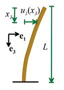The problem to be solved is illustrated in in the figure. A straight, vertical elastic cantilever beam with mass density $\rho$ and elastic modulus $E$ is clamped at its base and subjected to gravitational loading. The beam has length L, cross-sectional area A and principal moments of area $I_1,I_2,I_3$.  The straight, vertical rod is always an equilibrium configuration, but this configuration is stable only if $L<L_{crit}$.

 

Our objective is to show that the critical buckling length is

$L_{crit}\approx 2{\left({\displaystyle \frac{E{I}_2}{\rho Ag}}\right)}^{1/3}$

 

A number of different techniques can be used to find buckling loads.  One of the simplest procedures (which will be adopted here) is to identify the critical conditions where both the straight configuration (with $u_1=0$ ), and also the deflected configuration (with a small transverse deflection $u_1\ne 0$ ) are possible equilibrium shapes for the rod.

 

This problem can be solved using the governing equations for a beam subjected to large axial forces, listed in Section 10.3.3.    For the present case, we note that

 

1. The external forces acting on the rod are $p_1=0$, $p_3^{(e)}=\rho gA$, where g is the gravitational acceleration;

 

2. The acceleration is zero (because the rod is in static equilibrium)

 

3. The equilibrium equations therefore reduce to

$E{I}_2{\displaystyle \frac{d^4{u}_1}{d{x}_3^4}+\rho Ag{\displaystyle \frac{d{u}_1}{d{x}_3}=T_3{\displaystyle \frac{d^2{u}_1}{d{x}_3^2}}}}$          ${\displaystyle \frac{dN}{d{x}_3}+\rho Ag=0}$

 

4. These equations must be solved subject to the boundary conditions

$T_3=0,{\displaystyle \frac{d^2{u}_1}{d{x}_3^2}=0,{\displaystyle \frac{d^3{u}_1}{d{x}_3^3}=0x_3=0;u_1=0,{\displaystyle \frac{d{u}_1}{d{x}_3}=0x_3=L}}}$

 

5. Integrating the second equation of (3) and using the boundary condition $T_3=0$ at $x_3=0$ reduces the first equation of (3) to

$E{I}_2{\displaystyle \frac{d^4{u}_1}{d{x}_3^4}+\rho Ag{\displaystyle \frac{d{u}_1}{d{x}_3}+\rho Ag{x}_3{\displaystyle \frac{d^2{u}_1}{d{x}_3^2}=0}}}$

 

6. Integrating this equation with respect to $x_3$ and imposing the boundary condition $d^3{u}_1/d{x}_3^3=0$ at $x_3=0$ shows that

$E{I}_2{\displaystyle \frac{d^3{u}_1}{d{x}_3^3}+\rho Ag{x}_3{\displaystyle \frac{d{u}_1}{d{x}_3}=0}}$

 

7. This equation can be solved for $d{u}_1/d{x}_3$ using a symbolic manipulation program, which yields

${\displaystyle \frac{d{u}_1}{d{x}_3}=C_1{\mathrm{Ai}}_0\left[-x_3{\left({\displaystyle \frac{\rho Ag}{E{I}_2}}\right)}^{1/3}\right]+C_2{\mathrm{Bi}}_0\left[-x_3{\left({\displaystyle \frac{\rho Ag}{E{I}_2}}\right)}^{1/3}\right]}$

where ${\mathrm{Ai}}_0(x),{\mathrm{Bi}}_0(x)$ are special functions called `Airy Wave functions of order zero’

 

8. The remaining boundary conditions are $d{u}_1^2/d{x}_3^2=0$ at $x_3=0$, and $d{u}_1/d{x}_3=0$ at $x_3=L$.  Substituting (7) into the boundary conditions and writing the results in matrix form gives

$\left[\begin{array}{cc}{\mathrm{Ai}}_1(0)& {\mathrm{Bi}}_1(0)\\ {\mathrm{Ai}}_0(-\lambda )& {\mathrm{Bi}}_0(-\lambda )\end{array}\right]\left[\begin{array}{c}{C}_1\\ C_2\end{array}\right]=0$

where $\lambda =L{(\rho Ag/E{I}_2)}^{1/3}$ and ${\mathrm{Ai}}_1(x),{\mathrm{Bi}}_1(x)$ are Airy wave functions of order 1.

 

9. For this system of equations to have a nonzero solution, the determinant of the matrix must vanish, which shows that $\lambda$ must satisfy ${\mathrm{Ai}}_1(0){\mathrm{Bi}}_0(-\lambda )-{\mathrm{Bi}}_1(0){\mathrm{Ai}}_0(-\lambda )=0$.  This equation can easily be solved (numerically) for $\lambda$.  The smallest value of $\lambda$ that satisfies the equation is $\lambda \approx 2$.

 

10. The buckling length follows as

$L_{crit}\approx 2{\left({\displaystyle \frac{E{I}_2}{\rho Ag}}\right)}^{1/3}$

 

 

 

10.4.3  Post-buckled shape of an initially straight rod subjected to end thrust

 

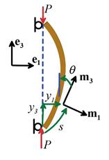The figure illustrates the problem to be solved.  An initially straight, inextensible elastic rod, with Young’s modulus E, length L and principal in-plane moments of area $I_1,I_2$  (with $I_2<I_1$ ) is subjected to end thrust.  The ends of the rod are constrained to travel along a line that is parallel to the undeformed rod, but the ends are free to rotate.   We wish to calculate the deformed shape of the rod.   You are probably familiar with the simple Euler buckling analysis that predicts the critical buckling loads.  Here, we derive the full post-buckling solution.

 

The rod is assumed to bow away from its straight configuration as shown: the deflected rod lies in the plane perpendicular to $e_2$.  The basis $\{m_1,m_2,m_3\}$ and the Euler angle $\theta$ that characterize the rotation of the rod’s cross sections are shown in the picture; the remaining Euler angles are $\psi =\varphi =0$.

 

Solution: Several possible equilibrium solutions may exist, depending on the applied load P.

 

1. The straight rod, with $\theta =y_2=0,x_3=s$ is always an equilibrium solution.  It is stable for applied loads $P<{\pi }^{2}E{I}_2/L^2$.

 

2. For applied loads $P>n^2{\pi }^{2}E{I}_2/L^2$, with n an integer, there are n+1 possible equilibrium solutions.  One of these is the straight rod; the rest are possible buckling modes.  The shape of each buckling mode depends on a parameter $k_n$ which satisfies

$L\sqrt{P/E{I}_2}=2nK(k_n)$

where K denotes a complete elliptic integral of the first kind

$K(k)={\displaystyle \underset{0}{\overset{\pi /2}{\int }}{(1-k^2{\sin }^{2}x)}^{-1/2}dx}$.

 Note that K has a minimum value $K=\pi /2$ at k=0, and increases monotonically to infinity as $k\to 1$.  The equation for $k_n$ has no solutions for $P<{\pi }^{2}E{I}_2/L^2$, and n solutions for $P>n^2{\pi }^{2}E{I}_2/L^2$, as expected.  If multiple solutions exist, only the solution with n=1 is stable.

 

3. The shape of the deformed rod can be characterized by the Euler angle $\theta$, which satisfies

$\theta =2{\sin }^{-1}\left\{\sqrt{k_n}sn\left(s\sqrt{(P/E{I}_2)}+K(k_n);k_n\right)\right\}$

where sn(x,k) denotes a Jacobi-elliptic function called the `sine-amplitude:’ its second argument k is called the `modulus’ of the function.

 

4. The coordinates of the buckled rod can also be calculated.  They are given by

$\begin{array}{l}{y}_3=-s+2\sqrt{E{I}_2/P}\left[{\rm E}\left(\text{am(}s\sqrt{P/E{I}_2}+K(k_n);k_n);k_n\right)-{\rm E}\left(\text{am(}K(k_n);k_n);k_n\right)\right]\\ y_2=-2\sqrt{k_{n}E{I}_2/P}\text{cn(}s\sqrt{P/E{I}_2}+K(k_n);k_n)\end{array}$

Here am(x,k) and cn(x,k) denote Jacobi elliptic functions called the `amplitude’ and `cosine amplitude’, and E(x,k) denotes an incomplete elliptic integral of the second kind

${\rm E}(x,k)={\displaystyle \underset{0}{\overset{x}{\int }}{(1-k^2{\sin }^{2}t)}^{1/2}dt}$.

The shape of the deflected rod for the stable buckling mode (n=1) is shown in the figure.

 

Derivation:  This is a large deflection problem and must be treated using the general equations listed in Sections 10.7-10.9.

 

1. The equilibrium equation $dT/ds=0$ immediately shows that T=constant along the rod’s length.  The boundary conditions at the end of the rod give $T=-P{e}_3$, so that the components of T in $\{m_1,m_2,m_3\}$ follow as $T_1=0,T_2=P\sin \theta ,T_3=-P\cos \theta$. 

 

2. Substituting the expressions for $T_i$ into the moment balance equations shows that $M_1=M_3=0$ and $d{M}_2/ds+P\sin \theta =0$

 

 

3. Finally, note that the curvatures are ${\kappa }_2=d\theta /ds,{\kappa }_1={\kappa }_3=0$, and recall that $M_2=E{I}_2{\kappa }_2$, so that the angle $\theta$ satisfies

$E{I}_2{\displaystyle \frac{d^2\theta }{d{s}^2}+P\sin \theta =0}$

 

4. This is the equation that governs oscillations of a pendulum, and its solution is well known. The equation is satisfied trivially by $\theta =0$ (this is the straight configuration), and also by two one-parameter families of functions of the form

$\theta =2{\sin }^{-1}\left\{\sqrt{k}sn\left((s-s_0)\sqrt{(P/E{I}_2)};k\right)\right\}\theta =2{\sin }^{-1}\left\{sn\left((s-s_0)\sqrt{(P/k^{2}E{I}_2)};k\right)\right\}$

Here, $s_0$ and $0<k<1$ are parameters whose values must be determined from the boundary conditions.  The first of these two functions is called an `inflexional’ solution, because the curve has points where $d\theta /ds=0$.  The second is called `non-inflexional’ because it has no such points.  For the pendulum, inflexional solutions correspond to periodic swinging motion; the non-inflexional solution corresponds to the pendulum whirling around the pivot. 

 

5. The bending moment must satisfy $M_2=0$ at both ends of the rod, which requires that $d\theta /ds=0$ at $s=0$ and $s=L$.  Only the inflexional solution can satisfy these boundary conditions.   For this case, we have

${\displaystyle \frac{d\theta }{ds}=2k\sqrt{{\displaystyle \frac{I_2}{P}}}cn\left((s-s_0)\sqrt{(P/E{I}_2)};k\right)}$

The cosine amplitude cn is a periodic function (it is a generalized cosine) and satisfies $cn(x,k)=0$ at $x=(2n+1)K(k)$.  We may therefore satisfy the boundary conditions by choosing

$-s_0\sqrt{P/E{I}_2}=K(k)$    and      $L\sqrt{P/E{I}_2}=2nK(k)$.

This leads to the defining equations for $k_n$.

 

6. Finally, the formula for the coordinates follows by integrating $d{y}_3/ds=\cos \theta$ and $d{y}_2/ds=\sin \theta$ subject to boundary conditions $y_1=0$ at $s=0,L$ and $y_3=0$ at s=0.

 

7. Finally, the (global) stability of the various solutions can be checked by comparing their potential energy.

 

 

 

 

10.4.4 Rod bent and twisted into a helix

 

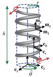
We consider an initially straight rod with length L, Young’s modulus E and shear modulus $\mu$.  The cross-section of the rod has area $A$, principal in-plane moments of inertia $I_1=I_2=I$ and an effective torsional inertia $J_3$.  The  rod is initially straight and unstressed, and is then subjected to forces and moments on its ends to bend and twist it into a helical shape, as shown in the figure. The geometry of the deformed rod can be characterized by:

 

1. The radius r of the cylinder that generates the helix

 

2. The total number of turns N in the helix

 

3. The helix angle $\alpha$, which is related to n and the height h of the helix by $\tan \alpha =h/(2\pi rN)$, and to the deformed length l of the rod by $\cos \alpha =2\pi rN/l$

 

4. The twist curvature ${\kappa }_3$, which quantify the distorsion induced by twisting the rod about its deformed axis.  For the rod to be in equilibrium, ${\kappa }_3$ must be constant.

 

5. The stretch ratio $\lambda =ds/d{x}_3$.  For the rod to be in equilibrium, $\lambda$ must be constant, and follows as $\lambda =l/L$.

 

 

The geometry and forces in the deformed rod are most conveniently described using a cylindrical-polar coordinate system $(r,\widehat{\theta },z)$ and basis $\left\{e_r,e_{\theta },e_3\right\}$ shown in Figure 10.15.  In terms of these basis vectors, we may define

 

1. The tangent vector to the rod $t=m_3=\cos \alpha e_{\theta }+\sin \alpha e_3$

 

2. The binormal vector is $b=-\sin \alpha e_{\theta }+\cos \alpha e_3$

 

 

In terms of these variables:

 

1. The internal moment in the rod is

$M=EI{\displaystyle \frac{{\cos }^2\alpha }{r}b+\mu J_3{\kappa }_3{m}_3}$

2. The internal force in the rod is

$T={\displaystyle \frac{{\cos }^2\alpha }{r}\left(\mu J_3{\kappa }_3-{\displaystyle \frac{EI}{r}\cos \alpha \sin \alpha }\right)b+EA(\lambda -1)m_3}$

For the limiting case of an inextensible rod, the quantity $EA(\lambda -1)$ should be replaced by an indeterminate axial force $T_3$.

 

 

The forces acting on the ends of the rod must satisfy $P=T$ and $Q=M$ at $s=L$ and $P=-T$ $Q=-M$ at s=0.

 

A variety of force and moment systems may deform the rod into a helical shape, depending on the twist and stretch.  An example of particular practical significance consists of a force $P=F_z{e}_3$ and moment $Q=r{F}_z{e}_{\theta }+Q_z{e}_z$ acting at s=L (with equal and opposite forces at s=0), where

$F_z={\displaystyle \frac{\cos \alpha }{r}(\mu J_3{\kappa }_3-{\displaystyle \frac{EI}{r}\cos \alpha \sin \alpha )Q_z=\mu J_3{\kappa }_3\sin \alpha +{\displaystyle \frac{EI}{r}{\cos }^3\alpha }}}$

This force system is statically equivalent to a wrench with force $F_z{e}_z$ and moment $Q_z{e}_z$ acting at r=0.

 

Finally note that this analysis merely gives conditions for a helical rod to be in static equilibrium.  The configuration may not be stable.

 

 

Derivation

 

1. We take $\widehat{\theta }=z=0$ at s=0, so that the cylindrical polar coordinates are related to arc-length by $\widehat{\theta }={\displaystyle \frac{s}{r}\cos \alpha z=s\sin \alpha }$. Note also that the basis vectors satisfy $d{e}_r/d\widehat{\theta }=e_{\theta }$, $d{e}_{\theta }/d\widehat{\theta }=-e_r$, so that

${\displaystyle \frac{d{e}_r}{ds}={\displaystyle \frac{\cos \alpha }{r}{e}_{\theta }}}$       ${\displaystyle \frac{d{e}_{\theta }}{ds}=-{\displaystyle \frac{\cos \alpha }{r}{e}_r}}$

 

2. The position vector of a point on the axis of the rod can be expressed as $r=r{e}_r+z{e}_3$;

 

3. The tangent vector follows as $m_3={\displaystyle \frac{dr}{ds}=\cos \alpha e_{\theta }+\sin \alpha e_3}$;

 

4. By definition, the curvature vector is

 

$\kappa =m_3\times {\displaystyle \frac{d{m}_3}{ds}+{\kappa }_3{m}_3=-{\displaystyle \frac{{\cos }^2\alpha \sin \alpha }{r}{e}_{\theta }+{\displaystyle \frac{{\cos }^3\alpha }{r}{e}_3+{\kappa }_3{m}_3}}}$

 which can be expressed in terms of the binormal vector as $\kappa =({\cos }^2\alpha /r)b+{\kappa }_3{m}_3$;

 

5. The moment-curvature relations then give the internal moment $M=EI({\cos }^2\alpha /r)b+\mu J_3{\kappa }_3{m}_3$;

 

6. The equilibrium equation $dT/ds+p=0$ shows that T=constant.  We may express this constant internal force vector in terms of its components as $T_r{e}_r+T_{\theta }{e}_{\theta }+T_z{e}_3$

 

7. The internal forces and moments must satisfy the moment equilibrium equation, which shows that

$\begin{array}{l}{\displaystyle \frac{dM}{ds}+m_3\times T={\displaystyle \frac{{\cos }^2\alpha }{r}\left({\displaystyle \frac{EI}{r}\cos \alpha \sin \alpha -J_3{\kappa }_3}\right)e_r+\mu J_3{\displaystyle \frac{d{\kappa }_3}{ds}(\cos \alpha e_{\theta }+\sin \alpha e_3)}}}\\ +\left(T_z\cos \alpha -T_{\theta }\sin \alpha \right)e_r+T_r\sin \alpha e_{\theta }-T_r\cos \alpha e_3=0\end{array}$

Taking the dot product of both sides of this equation with $m_3$ shows that $d{\kappa }_3/ds=0$. It then follows that $T_r=0$ and

${\displaystyle \frac{{\cos }^2\alpha }{r}\left(\mu J_3{\kappa }_3-{\displaystyle \frac{EI}{r}\cos \alpha \sin \alpha }\right)=\left(T_z\cos \alpha -T_{\theta }\sin \alpha \right)}$

 

8. Finally, the force-stretch relation requires that $T\cdot m_3=T_{\theta }\cos \alpha +T_z\sin \alpha =EA(\lambda -1)$.  This equation can be solved together with the final result of (7) for the components of internal force in the rod.

 

 

 

 

10.4.5 Helical spring

 

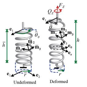The behavior of the helical spring shown in the figure can be deduced by means of a simple extension of the results in the preceding section. We assume that the spring is made from a material with shear modulus $\mu$ and Young’s modulus $E=2\mu (1+\nu )$.  The cross-section of the rod has principal in-plane moments of inertia $I_1=I_2=I$ and an effective torsional inertia $J$.  The rod is assumed to be inextensible, for simplicity.  The geometry of the undeformed spring can be characterized as follows:

 

1. The length of the rod L;

 

2. The radius $\overline{r}$ of the cylinder that generates the helix;

 

3. The height $\overline{h}$ of the spring;

 

4. The number of turns in the coil $N$;

 

5. The helix angle $\overline{\alpha }$.

 

The variables characterizing the undeformed spring are related as follows

$\tan \overline{\alpha }={\displaystyle \frac{\overline{h}}{2\pi \overline{r}N}\overline{h}=L\sin \overline{\alpha }}$

 

The spring is subjected to equal and opposite axial forces $F_z$ and axial twisting moments $Q_z$ at its ends, which act at the center of the cylinder generating the helix.   The precise manner in which the forces are transmitted to the ends of the helical rod is left unspecified, but we assume that the load points remain at the heights of the ends of the coil and remain at the center of the cylinder generating the helix.  In practice, this is always the case if the spring experiences only a small change in its shape, but (depending on how the spring is designed) large deflections may cause the applied forces to change their position or direction.   This would change the behavior of the spring.

 

Guided by the analysis in the preceding section, we anticipate that when the spring is deformed, it remains helical, and consequently can be characterized by the deformed radius $r$, the new height h and the new helix angle $\alpha$.   The load point at the top end of the spring may also rotate about the axis of the cylinder through an angle $\Delta \omega$.  It is of particular interest to relate the deflection $\Delta h$ and rotation $\Delta \omega$ to the force $F_z$ and axial moment $Q_z$.  

 

 

Solutions for small deflections and rotations of the spring

 

If a helical spring is subjected to small changes in its length $\Delta h<<\overline{h}$ (or small twisting rotations $\Delta \omega <<1$ ) the forces and twisting moment are proportional to $\Delta h$ and $\Delta \omega$. To give explicit formulas for spring stiffnesses, we assume in this section that the rod has a circular cross-section with diameter d, so that $J=2I=\pi d^4/32$.  The twist and extension are then related to the forces and moments by

$\left[\begin{array}{c}{F}_z\\ Q_z\end{array}\right]=\left[\begin{array}{cc}{k}_{Fh}& k_{F\omega }\\ k_{Qh}& k_{Q\omega }\end{array}\right]\left[\begin{array}{c}\Delta h\\ \Delta \omega \end{array}\right]\left[\begin{array}{c}\Delta h\\ \Delta \omega \end{array}\right]=\left[\begin{array}{cc}{c}_{hF}& c_{hQ}\\ c_{\omega F}& c_{\omega Q}\end{array}\right]\left[\begin{array}{c}{F}_z\\ Q_z\end{array}\right]$

where the stiffnesses and compliances are listed the table.

 

 

 

 

 

 

   We notice that:

 

· For practical values of pitch angle $\overline{\alpha }$ (which is typically less than 8 degrees) the stiffnesses can be approximated by

$k_{Fh}\approx {\displaystyle \frac{\mu d^4}{64{\overline{r}}^{3}N}{k}_{Q\omega }\approx {\displaystyle \frac{\mu (1+\nu )d^4}{64\overline{r}N}{k}_{Qh}=k_{F\omega }\approx 0}}$

These are the formulas that typically appear in design handbooks.  

 

· The extensional and rotational stiffnesses vary weakly with pitch angle $\overline{\alpha }$.   The stiffnesses and compliances are most significantly affected by the wire diameter and the radius of the coil.   Increasing the number of turns in the coil while keeping all other variables fixed will make the spring softer.

 

· For pitch angles exceeding about 20 degrees the coupling between rotation and axial force (or extension and torque) becomes significant.   As long as the spring deflection remains small, a spring with freely rotating ends will tend to uncoil as it is stretched.   A spring that is free of axial force will tend to extend when its ends are rotated.   In applications where this is undesirable two springs wound in opposite directions (one with a positive and a second with a negative pitch angle) are placed end-to end to cancel the rotation.

 

 

Solutions for large deflections and rotations of the spring

 

It is worth noting that the deformation in the helical part of a spring cannot be determined fully without knowing how the ends of the helical rod are connected to the force and moment acting on the coil.  The derivations shown in more detail below show that twisting the rod without changing the shape of the helix generates internal forces and moments in the rod that are statically equivalent to a vertical force and moment acting at the center of the coil.   Consequently, prescribing only the force and axial moment acting on the coil (or equivalently, prescribing the extension and rotation angle) is not sufficient to fully determine the deformation of the spring.  Furthermore, the forces acting on the spring may also depend on the history of deformation, since the ends of the rod may experience a sequence of rotations that generate a nonzero twist when the rod is returned to its original helical shape.  In the formulas given in this section, we have assumed that this does not occur. The force and moment acting on the spring are then given by

$-EI({\displaystyle \frac{{\cos }^2\alpha }{r}-{\displaystyle \frac{{\cos }^2\overline{\alpha }}{\overline{r}}){\displaystyle \frac{\sin \alpha }{r}+\mu J({\displaystyle \frac{\sin \alpha \cos \alpha }{r}-{\displaystyle \frac{\sin \overline{\alpha }\cos \overline{\alpha }}{\overline{r}}){\displaystyle \frac{\cos \alpha }{r}=F_z}}}}}}$

$EI({\displaystyle \frac{{\cos }^2\alpha }{r}-{\displaystyle \frac{{\cos }^2\overline{\alpha }}{\overline{r}})\cos \alpha +\mu J\left({\displaystyle \frac{\sin \alpha \cos \alpha }{r}-{\displaystyle \frac{\sin \overline{\alpha }\cos \overline{\alpha }}{\overline{r}}}}\right)\sin \alpha =Q{}_z}}$

where $\alpha$ and r are related to the height h of the deformed spring and the twist angle $\Delta \omega$ by

$h=L\sin \alpha L\left({\displaystyle \frac{\cos \alpha }{r}-{\displaystyle \frac{\cos \overline{\alpha }}{\overline{r}}}}\right)=\Delta \omega$

 

 

 

 

As an example, the force-extension relation and extension-rotation relation are plotted in the figure .   Results are shown for a spring with 10 turns and a Poisson ratio of $\nu =0.3$.  Fig (a) shows the normalized force and torque acting on a spring that is extended without twist; while Fig (b) shows the force and rotation of a spring that is extended while freely rotating.  The graphs show that:

 

· A spring with pitch angle less than 8 degrees remains linear for extensions exceeding 25% of the wire length.

 

· Springs with larger pitch angles tend to stiffen when extended, and soften when compressed.

 

· The torque acting on a spring that is prevented from rotating, and the twist of a freely rotating spring vary linearly with extension over only a narrow range of extension ( $\Delta h/L<0.05$).   Significant rotations (exceeding 20 degrees) can be expected if a freely rotating spring is stretched or compressed beyond 25% of the wire length.

 

 

Derivation: The geometry and forces in the spring are most conveniently described using a cylindrical-polar coordinate system $(r,\widehat{\theta },z)$ and basis $\left\{e_r,e_{\theta },e_3\right\}$ shown in Figure 10.16. 

 

1. We take $\widehat{\theta }=z=0$ at s=0, so that the cylindrical polar coordinates are related to arc-length by $\widehat{\theta }=(s/r)\cos \alpha z=s\sin \alpha$.

 

2. Note also that the basis vectors satisfy $d{e}_r/d\widehat{\theta }=e_{\theta }$, $d{e}_{\theta }/d\widehat{\theta }=-e_r$, so that

${\displaystyle \frac{d{e}_r}{ds}={\displaystyle \frac{\cos \alpha }{r}{e}_{\theta }}}$       ${\displaystyle \frac{d{e}_{\theta }}{ds}=-{\displaystyle \frac{\cos \alpha }{r}{e}_r}}$

 

3. The position vector of a point on the axis of the rod can be expressed as $r=r{e}_r+z{e}_3$;

 

4. The tangent vector follows as

$t=m_3={\displaystyle \frac{dr}{ds}=\cos \alpha e_{\theta }+\sin \alpha e_3}$;

 

5. The normal vector is

$n={\displaystyle \frac{1}{\left|{\displaystyle \frac{dt}{ds}}\right|}{\displaystyle \frac{dt}{ds}=-{\displaystyle \frac{\left({\cos }^2\alpha /r\right)e_r}{{\cos }^2\alpha /r}=-e_r}}}$

6. The binormal vector is $b=t\times n=\left(\cos \alpha e_{\theta }+\sin \alpha e_3\right)\times (-e_r)=-\sin \alpha e_{\theta }+\cos \alpha e_3$

 

7. It is helpful to select a basis $\left\{{\overline{m}}_1,{\overline{m}}_2,{\overline{m}}_3\right\}$ to characterize the orientation of the initial spring. As usual ${\overline{m}}_3=\overline{t}=\cos \overline{\alpha }{e}_{\theta }+\sin \overline{\alpha }{e}_3$ is tangent to the rod.   Since $I_1=I_2$ we may select ${\overline{m}}_1$ and ${\overline{m}}_2$ arbitrarily, as long as they are transverse to the rod’s axis. It is convenient to choose ${\overline{m}}_1$ and ${\overline{m}}_2$ to be parallel to the normal vector n and binormal vector b of the undeformed spring, respectively, which gives

${\overline{m}}_1=-e_r{\overline{m}}_2=-\sin \overline{\alpha }{e}_{\theta }+\cos \overline{\alpha }{e}_3{\overline{m}}_3=\cos \overline{\alpha }{e}_{\theta }+\sin \overline{\alpha }{e}_3$

 

8. The initial curvature of the rod can be calculated from the usual relation

$\begin{array}{l}{\displaystyle \frac{d{\overline{m}}_i}{ds}=\overline{\kappa }\times {\overline{m}}_i}\\ \Rightarrow {\displaystyle \frac{d{\overline{m}}_1}{ds}=-{\overline{\kappa }}_2{\overline{m}}_3+{\overline{\kappa }}_3{\overline{m}}_2{\displaystyle \frac{d{\overline{m}}_2}{ds}={\overline{\kappa }}_1{\overline{m}}_3-{\overline{\kappa }}_3{\overline{m}}_1{\displaystyle \frac{d{\overline{m}}_3}{ds}=-{\overline{\kappa }}_1{\overline{m}}_2+{\overline{\kappa }}_2{\overline{m}}_1}}}\end{array}$

This yields ${\overline{\kappa }}_1=0,{\overline{\kappa }}_2={\cos }^2\overline{\alpha }/\overline{r},{\overline{\kappa }}_3=\sin \overline{\alpha }\cos \overline{\alpha }/\overline{r}$, so that

$\overline{\kappa }={\displaystyle \frac{{\cos }^2\overline{\alpha }}{\overline{r}}{\overline{m}}_2+{\displaystyle \frac{\sin \overline{\alpha }\cos \overline{\alpha }}{\overline{r}}{\overline{m}}_3}}$

 

9. After deformation, the basis $\left\{{\overline{m}}_1,{\overline{m}}_2,{\overline{m}}_3\right\}$ rotates to a new basis $\left\{m_1,m_2,m_3\right\}$ aligned with the deformed rod.   Because the rod’s cross section is axially symmetric, and the rod is elastic, it is not necessary to assume that the basis vectors $m_1$ and $m_2$ (which are transverse to the bar) rotate with the rod’s twist.   Instead, we assume $m_1$ and $m_2$ remain parallel to the normal vector n and binormal vector b of the deformed spring, respectively, which gives $m_1=-e_r,m_2=-\sin \alpha e_{\theta }+\cos \alpha e_3,m_3=\cos \alpha e_{\theta }+\sin \alpha e_3$

 

10. The curvature vector of the deformed spring can therefore be expressed as

$\kappa ={\displaystyle \frac{{\cos }^2\alpha }{r}{m}_2+\left({\displaystyle \frac{\sin \alpha \cos \alpha }{r}+\Delta {\kappa }_3}\right)m_3}$

where $\Delta {\kappa }_3$ accounts for the rotation of the rod’s cross section about the tangent vector.  It cannot be determined from the orientation of $m_1$ and $m_2$ in the usual way, because they do not rotate with the bar’s cross-section.   If the axial force and moment acting on the spring are prescribed without any additional information specifying how the forces are connected to the ends of the helix (or equivalently, if only the extension and rotation or the spring are given) $\Delta {\kappa }_3$ is not uniquely determined: the detailed design of the portion of the spring that connects the helical coil to the external loading system would determine whether the rod’s cross section at the ends of the rod can twist about the rod’s center.   In all the following calculations, we shall assume that $\Delta {\kappa }_3=0$.   This means that at s=L the rod’s cross section has an angular velocity vector

$\omega ={\displaystyle \frac{d\alpha }{dt}{e}_r+{\displaystyle \frac{d\Delta \omega }{dt}\sin \alpha e_3}}$

as the spring is extended.  

 

11. The co-rotational rate of change of curvature (which quantifies the rate of change of twist and bending curvature relative to the basis vectors aligned with the deformed rod) is

$\stackrel{\nabla }{\kappa }={\displaystyle \frac{d}{dt}\left({\displaystyle \frac{{\cos }^2\alpha }{r}}\right)m_2+{\displaystyle \frac{d}{dt}\left({\displaystyle \frac{\sin \alpha \cos \alpha }{r}}\right)m_3}}$

 

12. The moment-curvature relations then give the internal moment

$\begin{array}{l}M=EI({\displaystyle \frac{{\cos }^2\alpha }{r}-{\displaystyle \frac{{\cos }^2\overline{\alpha }}{\overline{r}})b+\mu J\left({\displaystyle \frac{\sin \alpha \cos \alpha }{r}-{\displaystyle \frac{\sin \overline{\alpha }\cos \overline{\alpha }}{\overline{r}}}}\right)m_3}}\\ =EI({\displaystyle \frac{{\cos }^2\alpha }{r}-{\displaystyle \frac{{\cos }^2\overline{\alpha }}{\overline{r}})\left(-\sin \alpha e_{\theta }+\cos \alpha e_3\right)}}\\ +\mu J\left({\displaystyle \frac{\sin \alpha \cos \alpha }{r}-{\displaystyle \frac{\sin \overline{\alpha }\cos \overline{\alpha }}{\overline{r}}}}\right)\left(\cos \alpha e_{\theta }+\sin \alpha e_3\right)\end{array}$

 

13. The boundary conditions at the upper end of the spring relate the internal moment and force to the applied force

$M=-r{e}_r\times F_z{e}_3+Q{}_z{e}_3=r{F}_z{e}_{\theta }+Q{}_z{e}_{3}T=F_z{e}_3$

It is straightforward to show that this system of internal forces satisfies the equilibrium equation

${\displaystyle \frac{dM}{ds}+m_3\times T=0}$

which confirms our assumption that the spring remains helical after deformation.

 

 

14. Combining (9) and (10) shows that

$$\begin{array}{l}r{F}_z{e}_{\theta }+Q_z{e}_3=EI({\displaystyle \frac{{\cos }^2\alpha }{r}-{\displaystyle \frac{{\cos }^2\overline{\alpha }}{\overline{r}})\left(-\sin \alpha e_{\theta }+\cos \alpha e_3\right)}}\\ +\mu J\left({\displaystyle \frac{\sin \alpha \cos \alpha }{r}-{\displaystyle \frac{\sin \overline{\alpha }\cos \overline{\alpha }}{\overline{r}}}}\right)\left(\cos \alpha e_{\theta }+\sin \alpha e_3\right)\end{array}$$

This yields two equations relating the spring’s geometry to the external force and moment

$-EI({\displaystyle \frac{{\cos }^2\alpha }{r}-{\displaystyle \frac{{\cos }^2\overline{\alpha }}{\overline{r}}){\displaystyle \frac{\sin \alpha }{r}+\mu J\left({\displaystyle \frac{\sin \alpha \cos \alpha }{r}-{\displaystyle \frac{\sin \overline{\alpha }\cos \overline{\alpha }}{\overline{r}}}}\right){\displaystyle \frac{\cos \alpha }{r}=F_z}}}}$

$EI({\displaystyle \frac{{\cos }^2\alpha }{r}-{\displaystyle \frac{{\cos }^2\overline{\alpha }}{\overline{r}})\cos \alpha +\mu J\left({\displaystyle \frac{\sin \alpha \cos \alpha }{r}-{\displaystyle \frac{\sin \overline{\alpha }\cos \overline{\alpha }}{\overline{r}}}}\right)\sin \alpha =Q{}_z}}$

 

15. A final kinematic constraint relating the geometry of the spring to the motion of the load point can be found using the principle of virtual work.   Matching the internal and external rate of work gives

 

$\begin{array}{l}M\cdot \stackrel{\nabla }{\kappa }=L\left(r{F}_z{e}_{\theta }+Q_z{e}_3\right)\cdot \\ \left({\displaystyle \frac{d}{dt}({\displaystyle \frac{{\cos }^2\alpha }{r})\left(-\sin \alpha e_{\theta }+\cos \alpha e_3\right)+{\displaystyle \frac{d}{dt}\left({\displaystyle \frac{\sin \alpha \cos \alpha }{r}}\right)\left(\cos \alpha e_{\theta }+\sin \alpha e_3\right)}}}\right)\\ =Q_z{\displaystyle \frac{d\Delta \omega }{dt}+F_z{\displaystyle \frac{dh}{dt}}}\end{array}$

Comparing coefficients of F and Q shows that

$\begin{array}{l}-r{\displaystyle \frac{d}{dt}\left({\displaystyle \frac{{\cos }^2\alpha }{r}}\right)\sin \alpha +r{\displaystyle \frac{d}{dt}\left({\displaystyle \frac{\sin \alpha \cos \alpha }{r}}\right)\cos \alpha ={\displaystyle \frac{1}{L}{\displaystyle \frac{d\Delta h}{dt}}}}}\\ {\displaystyle \frac{d}{dt}\left({\displaystyle \frac{{\cos }^2\alpha }{r}}\right)\cos \alpha +{\displaystyle \frac{d}{dt}\left({\displaystyle \frac{\sin \alpha \cos \alpha }{r}}\right)\sin \alpha ={\displaystyle \frac{1}{L}{\displaystyle \frac{d\Delta \omega }{dt}}}}}\end{array}$

 

Hence

$\begin{array}{l}{\displaystyle \frac{d}{dt}\left({\displaystyle \frac{\sin \alpha \cos \alpha }{r}}\right)={\displaystyle \frac{1}{rL}{\displaystyle \frac{d\Delta h}{dt}\cos \alpha +{\displaystyle \frac{1}{L}{\displaystyle \frac{d\Delta \omega }{dt}\sin \alpha }}}}}\\ {\displaystyle \frac{d}{dt}\left({\displaystyle \frac{{\cos }^2\alpha }{r}}\right)=-{\displaystyle \frac{2\sin \alpha \cos \alpha }{r}{\displaystyle \frac{d\alpha }{dt}-{\displaystyle \frac{{\cos }^2\alpha }{r^2}{\displaystyle \frac{dr}{dt}=-{\displaystyle \frac{1}{Lr}{\displaystyle \frac{d\Delta h}{dt}\sin \alpha +{\displaystyle \frac{1}{L}{\displaystyle \frac{d\Delta \omega }{dt}\cos \alpha }}}}}}}}}\end{array}$

 

The results of steps 14 and 15 can be combined to calculate $F_z,Q_z$ for any given extension and rotation.   For example, the small deflection solution follows by setting

$\begin{array}{l}\left({\displaystyle \frac{\sin \alpha \cos \alpha }{r}-{\displaystyle \frac{\sin \overline{\alpha }\cos \overline{\alpha }}{\overline{r}}}}\right)={\displaystyle \frac{\Delta h}{rL}\cos \alpha +{\displaystyle \frac{\Delta \omega }{L}\sin \alpha }}\\ \left({\displaystyle \frac{{\cos }^2\alpha }{r}-{\displaystyle \frac{{\cos }^2\overline{\alpha }}{\overline{r}}}}\right)=-{\displaystyle \frac{\Delta h}{Lr}\sin \alpha +{\displaystyle \frac{\Delta \omega }{L}\cos \alpha }}\end{array}$

in (14), which shows that

$-EI\left(-{\displaystyle \frac{\Delta h}{Lr}\sin \alpha +{\displaystyle \frac{\Delta \omega }{L}\cos \alpha }}\right)\sin \alpha +\mu J\left({\displaystyle \frac{\Delta h}{rL}\cos \alpha +{\displaystyle \frac{\Delta \omega }{L}\sin \alpha }}\right)\cos \alpha =r{F}_z{e}_{\theta }$

$EI\left(-{\displaystyle \frac{\Delta h}{Lr}\sin \alpha +{\displaystyle \frac{\Delta \omega }{L}\cos \alpha }}\right)\cos \alpha +\mu J\left({\displaystyle \frac{\Delta h}{rL}\cos \alpha +{\displaystyle \frac{\Delta \omega }{L}\sin \alpha }}\right)\sin \alpha =Q{}_z$

Collecting terms and approximating $\alpha \approx \overline{\alpha },r\approx \overline{r}$ gives

${\displaystyle \frac{1}{L{\overline{r}}^2}\left(\mu J{\cos }^2\overline{\alpha }+EI{\sin }^2\overline{\alpha }\right)\Delta h+{\displaystyle \frac{1}{L\overline{r}}\left(\mu J-EI\right)\sin \overline{\alpha }\cos \overline{\alpha }\Delta \omega =F_z}}$

${\displaystyle \frac{1}{L\overline{r}}\left(\mu J-EI\right)\sin \overline{\alpha }\cos \overline{\alpha }\Delta h+{\displaystyle \frac{1}{L}\left(\mu J{\sin }^2\overline{\alpha }+EI{\cos }^2\overline{\alpha }\right)\Delta \omega =Q_z}}$

 

This yields the results listed in the table.