Chapter 1

 

Introduction $–$ Objectives and Applications of Solid Mechanics

 

 

Solid Mechanics is a collection of physical laws, mathematical techniques, and computer algorithms that can be used to predict the behavior of a solid material that is subjected to mechanical or thermal loading. The field has a wide range of applications, including

 

 

FEA model of a knee joint from the  MSC website.  They have several nice  FEA analysis movies

1.      Geomechanics $–$ modeling the shape of planets; tectonics; and earthquake prediction;

2.      Civil engineering $–$ designing foundations or structures;

3.      Mechanical engineering $–$ designing load bearing components for vehicles; power generation and transmission; 

4.      Manufacturing engineering $–$ designing metal and polymer forming processes; machining, etc;

5.      Biomechanics $–$ designing implants; bone mechanics; as well as modeling stress driven phenomena controlling celular and molecular processes;

6.      Materials Science $–$ designing composites; alloy microstructures, thin films, and developing materials processing;

7.      Microelectronics $–$ designing failure resistant packaging and interconnects;

8.      Nanotechnology $–$ stress driven self-assembly on surfaces; manufacturing processes such as nano-imprinting; modeling atomic-force microscope/sample interactions.

 

This chapter describes how solid mechanics can be used to solve practical problems.  The remainder of the book contains a more detailed description of the physical laws that govern deformation and failure in solids, as well as the mathematical and computational methods that are used to solve problems involving deformable solids. Specifically,

 

Chapter 2 covers the mathematical description of shape changes and internal forces in solids;

Chapter 3 discusses constitutive laws that are used to relate shape changes to internal forces;

Chapter 4 contains analytical solutions to a series of simple problems involving deformable solids;

Chapter 5 provides a short summary of analytical techniques and solutions for linear elastic solids;

Chapter 6 describes analytical techniques and solutions for plastically deforming solids;

Chapter 7 gives an introduction to finite element analysis, focusing on using commercial software;

Chapter 8 has a more complete discussion of the implementation of the finite element method;

Chapter 9 describes how to use solid mechanics to model material failure;

Chapter 10 discusses solids with special geometries (rods, beams, membranes, plates and shells).

 

Solid mechanics is incomprehensible without some background in vectors, tensors and index notation.  These topics are reviewed briefly in the appendices.

 

 

 

1.1 Defining a Problem in Solid Mechanics

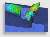
FEM simulation of chip formation during machining. From Third Wave Systems.

 

Regardless of the application, the general steps in setting up a problem in solid mechanics are always the same:

1.      Decide upon the goal of the problem and desired information;

2.      Identify the geometry of the solid to be modeled;

3.      Determine the loading applied to the solid;

4.      Decide what physics must be included in the model;

5.      Choose (and calibrate) a constitutive law that describes the behavior of the material;

6.      Choose a method of analysis;

7.      Solve the problem.

Each step in the process is discussed in more detail below.

 

 

 

1.1.1 Deciding what to calculate

 

An animation showing one of the vibration modes of the Mars Orbiter Laser Altimiter, from a NASA website.

This seems a rather silly question $–$ but at some point of their careers, most engineers have been told by their manager `Why don’t you just set up a finite element model of our (crank-case; airframe; material., etc, etc) so we can stop it from (corroding; fatiguing; fracturing, etc).’ If you find yourself in this situation, you are doomed. Models can certainly be helpful in preventing failure, but unless you have a very clear idea of why the failure is occurring, you won’t know what to model.

 

Here is a list of of some of the things that can typically be calculated very accurately using solid mechanics:

1.      The deformed shape of a structure or component subjected to mechanical, thermal or electrical loading;

2.      The forces required to cause a particular shape change;

3.      The stiffness of a structure or component;

4.      The internal forces (stresses) in a structure or component;

5.      The critical forces that lead to failure by structural instability (buckling);

FEA model of rupture during tube hydroforming.

6.      Natural frequencies of vibration for a structure or component.

 

In addition, solid mechanics can be used to model a variety of failure mechanisms.  Failure predictions are more difficult, however, because the physics of failure can only be modeled using approximate constitutive equations.  These must be calibrated experimentally, and do not always perfectly characterize the failure mechanism.  Nevertheless, there are well established procedures for each of the following:

 

1.      Predict the critical loads to cause fracture in a brittle or ductile solid containing a crack;

2.      Predict the fatigue life of a component under cyclic loading;

3.      Predict the rate of growth of a stress-corrosion crack in a component;

4.      Predict the creep life of a component;

5.      Find the length of a crack that a component can contain and still withstand fatigue or fracture;

6.      Predict the wear rate of a surface under contact loading;

7.      Predict the fretting or contact fatigue life of a surface.

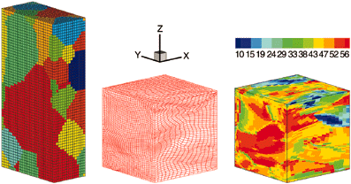
FEA model of the evolution of grain structure of a polycrystal during deformation.  From ORNL

 

Solid mechanics is increasingly being used for applications other than structural and mechanical engineering design.  These are active research areas, and some are better developed than others.  Applications include

 

1.      Calculating the properties (e.g. elastic modulus, yield stress, stress-strain curve; fracture toughness, etc) of a composite material in terms of those of its constituents.

2.      Predicting the influence of the microstructure (e.g. texture; grain structure; dispersoids; etc) on the mechanical properties of metals such as modulus, yield stress, strain hardening, etc.

3.      Modeling the physics of failure in materials, including fracture, fatigue, plasticity, and wear, and using the models to design failure resistant materials

4.      Modeling materials processing $–$ examples include casting and solidification; alloy heat treatments; thin film and surface coating deposition (e.g. by sputtering, vapor deposition or electroplating);

5.      Modeling biological phenomena and processes, such as bone growth; cell mobility; cell wall/particle interactions; and bacterial mobility.

 

 

 

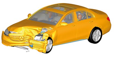
FEA crash simulation, from the ARUP LS DYNA website

1.1.2 Defining the geometry of the solid

 

Again, this seems rather obvious $–$ surely the shape of the solid is always known?  True $–$ but it is usually not obvious how much of the component to model, and at what level of detail.     For example, in a crash simulation, must the entire vehicle be modelled, or just the front part?  Should the engine block be included? The passengers? 

 

At the other extreme, it is often not obvious how much geometrical detail needs to be included in a computation.  If you model a component, do you need to include every geometrical feature (such as bolt holes, cutouts, chamfers, etc)?  The following guidelines might be helpful

 

1.      For modeling brittle fracture, fatigue failure, or for calculating critical loads required to initiate plastic flow in a component, it is very important to model the geometry in great detail, because geometrical features can lead to stress concentrations that initiate damage.

2.      For modeling creep damage, large scale plastic deformation (eg metal forming), or vibration analysis, geometrical details are less important.  Geometrical features with dimensions under 10% of the macroscopic cross section can generally be neglected.

3.      Geometrical features often only influence local stresses $–$ they do not have much influence far away.  Saint Venant’s principle, which will be discussed in more detail in Chapter 5, suggests that a geometrical feature with characteristic dimension L (e.g. the diameter of a hole in the solid) will influence stresses over a region with dimension around 3L surrounding the feature.  This means that if you are interested in the stress state at a particular point in an elastic solid, you need not worry about geometrical features that are far from the region of interest.  Saint-Venants principle strictly only applies to elastic solids, although it can usually also be applied to plastic solids that strain harden.

 

As a general rule, it is best to start with the simplest possible model, and see what it predicts.  If the simplest model answers your question, you’re done.  If not, the results can serve as a guide in refining the calculation

 

 

 

1.1.3 Defining loading

 

There are five ways that mechanical loads can be induced in a solid:

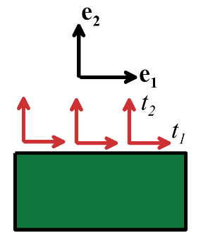
1.      The boundaries can be subjected to a prescribed displacement or motion;

2.      The boundaries can be subjected to a distribution of pressure normal to the surface, or frictional traction tangent to the surface;

3.      A boundary may be subjected to a combination of displacement and traction (“mixed”) boundary conditions $–$ for example, you could prescribe horizontal displacements, together with the vertical traction, at some point on the boundary;

4.      The interior of the solid can be subjected to gravitational or electromagnetic body forces;

5.      The solid can contact another solid, or in some cases can contact itself.

6.      Stresses can be induced by nonuniform thermal expansion in the solid, or some other materials process such as phase transformation that causes the solid to change its shape.

 

When specifying boundary conditions, you must follow these rules:

1.      In a 3D analysis, you must specify three components of either displacement $(u_1,u_2,u_3)$ or traction $\left(t_1,t_2,t_3\right)$ (but not both) at each point on the boundary.  You can mix these $–$ so for example you could prescribe $(u_1,t_2,t_3)$ or $(u_1,u_2,t_3)$, but exactly three components must always be prescribed. This includes free surfaces, where the tractions are prescribed to be zero.

2.      Similarly, in a 2D analysis you must prescribe two components of displacement or traction at each point on the boundary.

3.      If you are solving a static problem with only tractions prescribed on the boundary, you must ensure that the total external force acting on the solid sums to zero (otherwise a static equilibrium solution cannot exist).

 

In practice, it can be surprisingly difficult to find out exactly what the loading on your system looks like.  For example, earthquake loading on a building can be modeled as a prescribed acceleration of the building’s base $–$ but what acceleration should you apply?  Pressure loading usually arises from wind or fluid forces, but you might need to do some sophisticated calculations just to identify these forces.  In the case of contact loading, you’ll need to be able to estimate friction coefficients.  For nano-scale or biological applications, you may also need to model attractive forces between the two contacting surfaces.

 

This is where standards are helpful.  For example, building codes regulate civil engineernig structures; NHTSA specify design requirements for vehicles, and so on. 

 

You can also avoid the need to find exactly what loading a structure will experience in service by simply calculating the critical loads that will lead to failure, or the fatigue life as a function of loading.  In this case some other unfortunate engineer will have to decide whether or not the failure loads are acceptable.

 

 

 

1.1.4 Deciding what physics to include in the model

 

There are three decisions to be made here:

 

1.      Do you need to calculate additional field quantities, such as temperature, electric or magnetic fields, or mass/fluid diffusion through the solid?  Temperature is the most common additional field quantity. Here are some rough guidelines that will help you to decide whether to account for heating effects.

 

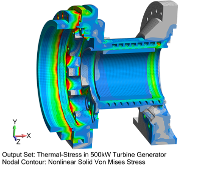
As a rough guide, the stress induced by temperature variation in a component is $\sigma =E{(\alpha T)}_{\max }-{(\alpha T)}_{\min })$, where E is the Young’s modulus of the material; $\alpha$ is its thermal expansion coefficient, and T is temperature. The symbols ${\left(\alpha T\right)}_{\max },{\left(\alpha T\right)}_{\min }$ denote the maximum and minimum values of the product $\alpha T$ in the component.  You need to account for temperature variations if $\sigma$ is a significant fraction of the stress induced by mechanical loading.

 

Thermal stress analysis of a turbine casing, from the consulting firm IDAC

To decide whether you need to do a transient heat conduction analysis, note that the temperature rise at a distance r from a point source of heat of intensity $\dot{Q}$ in an infinite solid is $\Delta T=\dot{Q}\text{erfc}\left(r/2\sqrt{\alpha t}\right)/\left(4\pi \kappa r\right)$, where erfc() denotes the complementary error function, $\kappa$ is the material’s thermal conductivity, and $\chi =\kappa /(\rho c_p)$ is its thermal diffusivity, with $\rho$ the mass density and $c_p$ the specific heat capacity. This suggests that a solid with dimension L will reach its steady state temperature in time $t\approx 25L^2/\chi$.  If the time-scale of interest in your problem is significantly larger than this, and heat flux is contstant, you can use the steady-state temperature distribution.  If not, you must account for transients.

 

Finally to decide whether you need to account for heat generated by plastic flow, note that the rate of heat generation per unit volume is of order $\dot{q}={\sigma }_Y{\dot{\epsilon }}^p$ where ${\sigma }_Y$ is the material yield stress, and ${\dot{\epsilon }}^p$ is the plastic strain rate.  The temperature rise due to rapid (adiabatic) plastic heating is thus of order $\Delta T={\sigma }_Y\Delta {\epsilon }^p/(\rho c_p)$, where $\Delta {\epsilon }^p$ is the strain increment applied to the material.

 

A dynamic analysis of a leg kicking a soccer ball. From the Fluent website

2.      Do you need to do a dynamic analysis, or a static analysis?  Here are some rough guidelines that will help you to decide:

The speed of a shear wave propagating through an elastic solid is $c=\sqrt{\mu /\rho }$, where $\rho$ is the mass density of the solid, $\mu$ is its shear modulus and $\nu$ its Poisson’s ratio.  The time taken for a wave to propagate across a component with size L is of order $t=L/c$.  In many cases, stresses decay to their static values after about 10L/c.  If the loading applied to the component does not change significantly during this time period a quasi-static computation (possibly including accelerations as body forces) should suffice.

The stress induced by acceleration (e.g. in a rotating component) is of order $L\rho a$, where L is the approximate size of the component, $\rho$ is its mass density, and a is the magnitude of the acceleration.  If this stress is negligible compared with other forces applied to the solid, it can be neglected.  If not, it should be included (as a body force if wave propagation can be neglected).

A coupled fluid-solid analysis from CEI

 

3.      Are you solving a coupled fluid/solid interaction problem?  These arise in aeroelasticity (design of flexible aircraft wings or helicopter rotor blades; or very long bridges); offshore structures; pipelines; or fluid containers.  In these applications the fluid flow has a high Reynold’s number (so fluid forces are dominated by inertial effects).  Coupled problems are also very common in biomedical applications such as blood flow or cellular mechanics. In these applications the Reynolds number for the fluid flow is much lower, and fluid forces are dominated by viscous effects.  Different analysis techniques are available for these two applications. Such problems are beyond the scope of this book.

 

 

 

1.1.5 Defining material behavior

 

Choosing the right equations to describe material behavior is the most critical part of setting up a solid mechanics calculation.  Using the wrong model, or inaccurate material properties, will always completely invalidate your predictions.  Here are a few of your choices, with suggested applications:

 

FEA model of a rubber tire, using a hyperelastic constitutive equation. From the LOZIK website

1.      Isotropic linear elasticity (familiar in one dimension as $\sigma =E\epsilon$ ) $–$ good for polycrystalline metals, ceramics, glasses, and polymers udergoing small deformations and subjected to low loads (less than the material yield stress).  Only two material constants are required to characterize the material, and material data is highly accurate and readily available.

 

2.      Anisotropic linear elasticity (similar to isotropic linear elasticity, but models materials which are stiffer in some directions than others). Good for reinforced composites; wood; single crystals of metals and ceramics.  Between 3 and 21 material properties must be determined. Material data is highly accurate and readily available.Isotropic or anisotropic linear elasticity is good for the vast majority of engineering design calculations, where components cannot safely exceed yield.  It can be used for deflection calculations, fatigue analysis, and vibration analysis.

 

3.      `Hyperelasticity’ $–$ used to model rubber and foams, which can sustain huge, reversible, shape changes.  There are several models to choose from.  The simplest model (the incompressible Neo-Hookean solid, which, in uniaxial stress,  has a true stress $–$ true strain relation given by $\sigma =C(\exp (2\epsilon )-1/\exp (\epsilon ))$ ) has only a single material constant.  More complex models have several parameters, and it may be difficult to find values for your material in the published literature.  Experimental calibration will almost certainly be required.

FEA model of a die-forming process, from the DIPRO website.  A sophisticated plasticity model would be required to accurately predict the wall-thickness of the part and its elastic springback.

 

4.      Viscoelasticity. Used to model materials which exhibit a gradual increase in strain when loaded at constant stress (with stress rate-v-strain rate $\dot{\epsilon }=\dot{\sigma }/E+\eta \sigma$ ) or which show hysteresis during cyclic loading (with stress-v-strain rate of form  $\sigma =E\epsilon +\lambda \dot{\epsilon }$ ).   Usually used to model polymeric materials and polymer based composites, and biological tissue.   Can also model slow creep in amorphous solids such as glass.  Constitutive equations contain at least 3 parameters, and usually many more. Material behavior varies widely between materials and is highly temperature dependent.  Experimental calibration will almost certainly be required to obtain accurate predictions.

 

 

5.      Rate independent metal plasticity.  Used to model permanent deformation in metals loaded above their yield point.  A wide range of models are available.  The simplest  is a rigid perfectly plastic solid, which changes its shape only if loaded above its yield stress ${\sigma }_Y$, and then deforms at constant stress.  An elastic-perfectly plastic solid deforms according to linear elastic equations when loaded below the yield stress, but deforms at constant stress if yield is exceeded.  These models would be appropriate to predict energy dissipation in a crash analysis, or to calculate tool forces in a metal cutting operation, for example. Data for material yield stress are readily available, but are sensitive to material processing and microstructure and so should be used with caution. More sophisticated models describe strain hardening in some way (the change in the yield stress of the solid with plastic deformation).   These are used in modeling ductile fracture, low cycle fatigue (where the material is repeatedly plastically deformed), and when predicting residual stresses and springback in metal forming operations. Finally, the most sophisticated plasticity models attempt to track the development of microstructure or damage in the metal.  For example, the Gurson plasticity model (developed at Brown University by then-graduate student A.L Gurson) models the nucleation and growth of voids in a metal, and is widely used to simulate ductile fracture.  Such models typically have a large number of parameters, and can  differ widely in their predictions. They must be very carefully chosen and calibrated to get good results.

 

FEA simulation of fracture in a weld using a Gurson platicity model, which accounts for ductile rupture by void nucleation and growth.  From the NW numerics website

6.      Viscoplasticity: similar in structure to metal plasticity, but accounts for the tendency of the flow stress of a metal to increase when deformed at high strain rates.   These would be used in modeling high-speed machining, for example, or in applications involving explosive shock loading.  Viscoplastic constitutive equations are also used to model creep $–$ the steady accumulation of plastic strain in a metal when loaded below its yield stress, and subjected to high temperatures.  The simplest viscoplastic constitutive law has  a uniaxial strain rate versus stress response of the form $\dot{\epsilon }=A{\sigma }^n$ and so has only two parameters.  More complex models account for elastic deformation and strain hardening.  Data for the simple models is quite easy to find, but more sophisticated and accurate models would have to be calibrated experimentally.

 

7.      Crystal plasticity:  Used to model anisotropic plastic flow in a single crystal of a metal.  Mostly used in materials science calculations and in modeling some metal forming processes.  These models are still under development, material data is not easy to find, and very laborious and expensive to measure.

 

8.      Strain Gradient Plasticity: A formulation developed in the last 5-10 years to model the behavior very small volumes of a metal (i.e. less than 100 $\mu m$ ).  Typically, small volumes of metal are stronger than bulk samples.  These models are still under development, are difficult to calibrate, and don’t always work very well.

 

9.       Discrete Dislocation Plasticity: A technique to model plastic flow in very small volumes of material by tracking the nucleation, motion and annihiliation of individual dislocations in the solid.  DDP models contain a large number of material parameters that are very hard to calibrate. Currently a research tool.

 

Discrete dislocation plasticity simulation of dislocations near the tip of a propagating crack.  From the GM/Brown CRL website.

10.  Critical state plasticity (cam-clay).  Used to model soils, whose behavior depends on moisture content.  Somewhat similar in structure to metal plasticity, except that the yield strength of a soil is highly pressure dependent (it increases with compressive pressure).  Simple models contain only 3 or 4 material parameters that can be calibrated quite accurately.

 

11.  Pressure-dependent viscoplasticity.  Similar to critical state plasticity, in that these models account for changes in flow stress of a material with confining pressure.  Used to model granular materials, and some polymers and composite materials (typically in modeling processes such as extrusion or drawing).

 

12.  Concrete models. Intended to model the crushing (in compression) or fracture (in tension) of concrete (obviously!). The mathematical structure resembles that of pressure dependent plasticity.

 

Quasicontinuum simulation of a crack approaching a bi-material interface.  From the Quasicontinuum website.

13.  Atomistic models. Replace traditional stress-strain laws with a direct calculation of stress-strain behavior using embedded atomic scale simulations.  The atomic scale computations use empirical potentials to model atom interactions, or may approximate the Schrodinger wave equation directly. Techiques include the `Quasi-Continuum’ method, and the Coupled-Atomistic-Discrete Dislocation Method. Their advantage is that they capture the physics of material behavior extremely accurately; their disadvantage is that they currently can only model extremely small material volumes (20-100nm or so). Atomistic models based on empirical potentials contain a large number of adjustable parameters $–$ these are usually calibrated against known quantities such as elastic moduli and stacking fault energies, and can also be computed using ab-initio techniques.  The accuracy of the the predictions depends strongly on the accuracy of the potentials. Mostly a research tool for nanotechnology and materials design applications.

 

This is by no means an exhaustive list $–$ additional models are available for materials such as shape memory alloys, and piezoelectric materials, for example.

 

These material models are intended primarily to approximate stress-strain behavior.  Special constitutive equations have also been developed to model the behavior of contacting surfaces or interfaces between two solids (Coulomb friction is a simple example). In addition, if you need to model damage (fracture or fatigue), you may need to select and calibrate additional material models.  For example, to model brittle fracture, you would need to know the fracture toughness of the material.  To model the growth of a fatigue crack, you would probably use Paris’ grack growth law  $da/dt=C{\left(\Delta K\right)}^n$ and would need data for the Paris constant C and exponent n.  There are several other stress- or strain-based fatigue laws in common use.  These models are often curve fits to experimental data, and are not based on any detailed physical understanding of the failure mechanism.  They must therefore be used with caution, and material properties must be measured carefully.

 

 

 

1.1.6 A representative initial value problem in solid mechanics

 

The result of the decisions made in Sections 1.1.1-1.1.5 is a Boundary value problem (for static problems) or initial value problem (for dynamic problems).  This consists of a set of partial differential equations, together with initial and boundary conditions, that must be solved for the displacement and stress fields, as well as any auxiliary fields (such as temperature) in the solid.   To illustrate the structure of these equations, in this section we list the governing equations for a representative initial value problem.

 

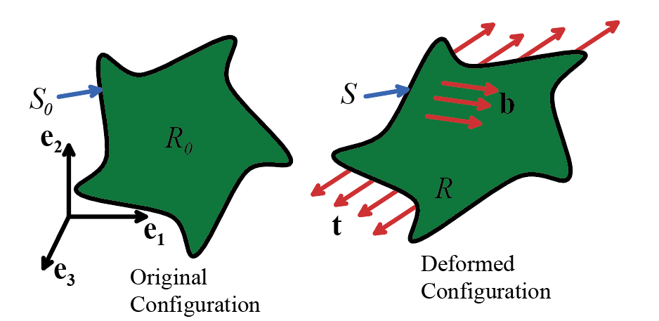
As a representative example, we state the initial value problem that governs elastic wave propagation in a linear elastic solid.

 

Given:

1.      The shape of the solid in its unloaded condition $R$

2.      The Young’s modulus E and Poisson’s ratio $\nu$ for the solid

3.      The thermal expansion coefficient $\alpha$ for the solid, and temperature distribution $T(x)$ in the solid (for simplicity we assume that the temperature does not vary with time)

4.      The initial displacement field in the solid $\stackrel{o}{u}(x)$, and the initial velocity field $\stackrel{o}{v}(x)$

5.      A body force distribution $b(x,t)$ (force per unit volume) acting on the solid

6.      Boundary conditions, specifying displacements $u^{*}(x,t)$ on a portion ${\partial }_{1}R$ and  tractions $t^{*}(x,t)$ on a portion ${\partial }_{2}R$ of the boundary of R

 

Calculate displacements $u_i$, strains ${\epsilon }_{ij}$ and stresses ${\sigma }_{ij}$ satisfying the governing equations of linear elastodynamics:

1.      The strain-displacement (compatibility) equation ${\epsilon }_{ij}=\frac{1}{2}(\partial u_i/\partial x_j+\partial u_j/\partial x_i)$

2.      The linear elastic stress-strain law ${\sigma }_{ij}=\frac{E}{1+\nu }\left({\epsilon }_{ij}+\frac{\nu }{1-2\nu }{\epsilon }_{kk}{\delta }_{ij}\right)-\frac{E\nu }{(1+\nu )(1-2\nu )}\alpha \Delta T{\delta }_{ij}$

3. The equation of motion for a continuum (F=ma) $\partial {\sigma }_{ij}/\partial x_i+b_j=\rho {\partial }^2{u}_j/\partial t^2$

4.      The fields must satisfy initial conditions $u_i(x_i,t=0)=\stackrel{0}{u_i}\frac{\partial u_i(x_i,t=0)}{\partial t}=\stackrel{0}{v_i}$

5.      As well as boundary conditions $\begin{array}{l}{u}_i=u_i^{*}(x_k,t)\text{on}{\partial }_{1}R\\ {\sigma }_{ij}{n}_i=t_j^{*}(x_k,t)\text{on}{\partial }_{2}R\end{array}$

 

 

 

1.1.7 Choosing a method of analysis

 

Once you have set up the problem, you will need to solve the equations of motion (or equilibrium) for a continuum, together with the equations governing material behavior, to determine the stress and strain distributions in the solid.  Several methods are available for this purpose.

 

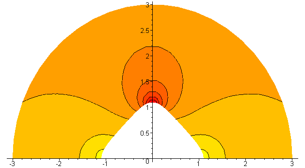
Exact solutions: There is a good chance that you can find an exact solution for:

Analytical solution to the stress field around a hypotrochoidal hole in an elastic solid

1.      2D (plane stress or plane strain) linear elastic solids, particularly under static loading.  Solution techniques include transforms, stress function methods, and complex variable methods. Dynamic solutions are also possible, but somewhat more difficult.

2.      2D viscoelastic solids.

3.      3D linear elasticitity problems can be solved, usually using integral transforms, if they are simple enough.

4.      2D (plane strain) deformation of rigid plastic solids (using slip line fields)

 

Naturally, analytical solutions are most easily found for solids with a simple geometry (e.g. an infinite solid containing a crack; loading applied to a flat surface, etc).  In addition, special analytical techniques can be used for problems where the solid’s geometry can be approximated in some way.  Examples include membrane theory; shell and plate theory; beam theory; and truss analysis.

 

Even when you can’t find an exact solution to the stress and strain fields in your solid, you can sometimes get the information you need using powerful mathematical theorems.  For example, bounding theorems allow you to estimate the plastic collapse loads for a structure quickly and easily. 

 

Numerical Solutions: These are used for most engineering design calculations in practice. These include

1.      The finite element method $–$ which will be discussed in detail in this book.  This is the most widely used technique, and can be used to solve almost any problem in solid mechanics, provided you understand how to model your material, and have access to a fast enough computer.

2.      Finite difference methods $–$ somewhat similar to FEM but much less widely used. 

3.      The boundary integral equation method (or boundary element method) is a more efficient computer technique for linear elastic problems, but is less well suited to nonlinear materials or geometry.

4.      Free volume methods: Used more in computational fluid dynamics than in solids, but good for problems involving very large deformations, where the solid flows much like a fluid.

5.      Atomistic methods: used in nanotechnology applications to model material behavior at the atomic scale.  Molecular Dynamic techniques integrate the equations of motion (Newton’s laws) for individual atoms; Molecular statics solve equilibrium equations to calculate atom positions.  The forces between atoms are computed using empirical constitutive equations, or sometimes using approximations to quantum mechanics.  These computations can only consider exceedingly small material volumes (up to a few million atoms) and short time-scales (up to a nanosecond).