2.4 Equations of motion and equilibrium for deformable solids

 

In this section, we generalize the laws of mass conservation, conservation of linear and angular momentum) to a deformable solid.

 

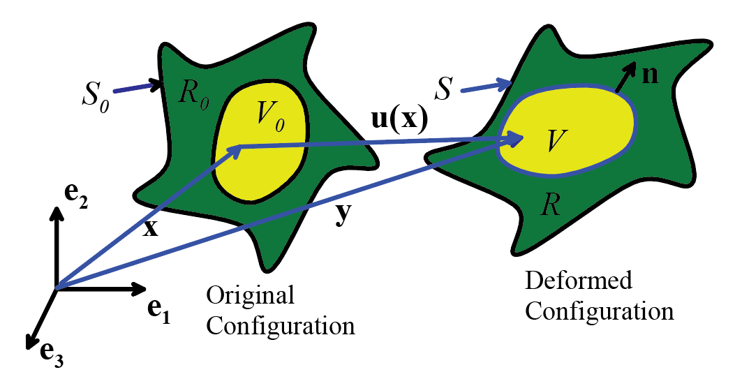
2.4.1 Mass Conservation

 

The total mass of any subregion V (as shown in the figure) within a deformable solid must be conserved.  We can write express this condition as a constraint in several different ways.  The rate of change of total mass within V must be zero, so that

${\displaystyle \frac{d}{dt}{\displaystyle \underset{V}{\int }\rho (y,t)dV}=\text{0}}$

where $\rho$ is the mass density in the deformed solid.  Or, (using Reynolds transport relation, proved in Section 2.2.27) we can write a local mass conservation equation, which relates the rate of change of mass density to the velocity gradient

${\displaystyle \underset{V}{\int }\left({\left.{\displaystyle \frac{\partial \rho }{\partial t}}\right|}_{x=const}+\rho {\displaystyle \frac{\partial v_i}{\partial y_i}}\right)}dV=0\Rightarrow {\left.{\displaystyle \frac{\partial \rho }{\partial t}}\right|}_{x=const}+\rho {\displaystyle \frac{\partial v_i}{\partial y_i}=0}$

 

 

The Eulerian version of the mass conservation equation is more common in fluid mechanics

${\left.{\displaystyle \frac{\partial \rho }{\partial t}}\right|}_{y=const}+{\displaystyle \frac{\partial \rho v_i}{\partial y_i}=0}$

 

 

 

 

 

 

 

2.4.2 Linear momentum balance in terms of Cauchy stress

 

Consider a solid that is deformed by external forces, as shown in the figure. Let ${\sigma }_{ij}$ denote the Cauchy stress distribution within a deformed solid.  Assume that the solid is subjected to a body force $b_i$, and let $u_i,v_i$ and $a_i$ denote the displacement, velocity and acceleration of a material particle at position $y_i$  in the deformed solid.

 

Newton’s third law of motion (F=ma) can be expressed as

${\nabla }_y\cdot \sigma +\rho b=\rho a\text{ or }{\displaystyle \frac{\partial {\sigma }_{ij}}{\partial y_i}+\rho b_j=\rho a_j}$

Written out in full

$\begin{array}{l}{\displaystyle \frac{\partial {\sigma }_{11}}{\partial y_1}+{\displaystyle \frac{\partial {\sigma }_{21}}{\partial y_2}+{\displaystyle \frac{\partial {\sigma }_{31}}{\partial y_3}+\rho b_1=\rho a_1}}}\\ {\displaystyle \frac{\partial {\sigma }_{12}}{\partial y_1}+{\displaystyle \frac{\partial {\sigma }_{22}}{\partial y_2}+{\displaystyle \frac{\partial {\sigma }_{32}}{\partial y_3}+\rho b_2=\rho a_2}}}\\ {\displaystyle \frac{\partial {\sigma }_{13}}{\partial y_1}+{\displaystyle \frac{\partial {\sigma }_{23}}{\partial y_2}+{\displaystyle \frac{\partial {\sigma }_{33}}{\partial y_3}+\rho b_3=\rho a_3}}}\end{array}$

Note that the derivative is taken with respect to position in the actual, deformed solid. For the special (but rather common) case of a solid in static equilibrium in the absence of body forces

${\displaystyle \frac{\partial {\sigma }_{ij}}{\partial y_i}=0}$

 

Derivation: Recall that the resultant force acting on an arbitrary volume of material V within a solid is

$P_i={\displaystyle \underset{A}{\int }{T}_i(n)dA+}{\displaystyle \underset{V}{\int }\rho b_{i}dV}$

where T(n) is the internal traction acting on the surface A with normal n that bounds V.

 

The linear momentum of the volume V is

${\Lambda }_i={\displaystyle \underset{V}{\int }\rho v_i}dV$

where v is the velocity vector of a material particle in the deformed solid. Express T in terms of ${\sigma }_{ij}$ and set $P_i=d{\Lambda }_i/dt$. Then

${\displaystyle \underset{A}{\int }{\sigma }_{ji}{n}_{j}dA+}{\displaystyle \underset{V}{\int }\rho b_{i}dV}={\displaystyle \frac{d}{dt}\left\{{\displaystyle \underset{V}{\int }\rho v_i}dV\right\}}$

Apply the divergence theorem to convert the first integral into a volume integral, and note that one can show (see Appendix E) that

${\displaystyle \frac{d}{dt}\left\{{\displaystyle \underset{V}{\int }\rho v_i}dV\right\}={\displaystyle \underset{V}{\int }\rho a_i}dV}$

So

${\displaystyle \underset{V}{\int }{\displaystyle \frac{\partial {\sigma }_{ji}}{\partial y_j}dV+}}{\displaystyle \underset{V}{\int }\rho b_{i}dV}={\displaystyle \underset{V}{\int }\rho a_i}dV\Rightarrow {\displaystyle \underset{V}{\int }\left({\displaystyle \frac{\partial {\sigma }_{ji}}{\partial y_j}+\rho b_i-\rho a_i}\right)}dV=0$

Since this must hold for every volume of material within a solid, it follows that

${\displaystyle \frac{\partial {\sigma }_{ji}}{\partial y_j}+\rho b_i=\rho a_i}$

as stated.

 

 

 

2.4.3 Angular momentum balance in terms of Cauchy stress

 

Conservation of angular momentum for a continuum requires that the Cauchy stress satisfy

${\sigma }_{ji}={\sigma }_{ij}$

i.e. the stress tensor must be symmetric.

 

Derivation: write down the equation for balance of angular momentum for the region V within the  deformed solid

${\displaystyle \underset{A}{\int }y\times TdA}+{\displaystyle \underset{V}{\int }y\times \rho bdV}={\displaystyle \frac{d}{dt}\left\{{\displaystyle \underset{V}{\int }y\times \rho vdV}\right\}}$

Here, the left hand side is the resultant moment (about the origin) exerted by tractions and body forces acting on a general region within a solid.  The right hand side is the total angular momentum of the solid about the origin.

 

We can write the same expression using index notation

${\displaystyle \underset{A}{\int }{\in }_{ijk}{y}_j{T}_{k}dA}+{\displaystyle \underset{V}{\int }{\in }_{ijk}{y}_j{b}_k\rho dV}={\displaystyle \frac{d}{dt}\left\{{\displaystyle \underset{V}{\int }{\in }_{ijk}{y}_j{v}_k\rho dV}\right\}}$

Express T in terms of ${\sigma }_{ij}$ and re-write the first integral as a volume integral using the divergence theorem

$\begin{array}{l}{\displaystyle \underset{A}{\int }{\in }_{ijk}{y}_j{T}_{k}dA}={\displaystyle \underset{A}{\int }{\in }_{ijk}{y}_j{\sigma }_{mk}{n}_{m}dA}={\displaystyle \underset{V}{\int }{\displaystyle \frac{\partial }{\partial x_m}\left({\in }_{ijk}{y}_j{\sigma }_{mk}\right)dV}}\\ ={\displaystyle \underset{V}{\int }{\in }_{ijk}\left({\delta }_{jm}{\sigma }_{mk}+y_j{\displaystyle \frac{\partial {\sigma }_{mk}}{\partial x_m}}\right)dV}\end{array}$

We may also show (see Appendix E) that

${\displaystyle \frac{d}{dt}\left\{{\displaystyle \underset{V}{\int }{\in }_{ijk}{y}_j{v}_k\rho dV}\right\}={\displaystyle \underset{V}{\int }{\in }_{ijk}{y}_j{a}_k\rho dV}}$

Substitute the last two results into the angular momentum balance equation to see that

$\begin{array}{l}{\displaystyle \underset{V}{\int }{\in }_{ijk}\left({\delta }_{jm}{\sigma }_{mk}+y_j{\displaystyle \frac{\partial {\sigma }_{mk}}{\partial x_m}}\right)dV}+{\displaystyle \underset{V}{\int }{\in }_{ijk}{y}_j{b}_k\rho dV}={\displaystyle \underset{V}{\int }{\in }_{ijk}{y}_j{a}_k\rho dV}\\ \Rightarrow {\displaystyle \underset{V}{\int }{\in }_{ijk}{\delta }_{jm}{\sigma }_{mk}=-}{\displaystyle \underset{V}{\int }{\in }_{ijk}{y}_j\left({\displaystyle \frac{\partial {\sigma }_{mk}}{\partial y_m}+\rho b_k-\rho a_k}\right)dV}\end{array}$

The integral on the right hand side of this expression is zero, because the stresses must satisfy the linear momentum balance equation.  Since this holds for any volume V, we conclude that

$\begin{array}{l}{\in }_{ijk}{\delta }_{jm}{\sigma }_{mk}={\in }_{ijk}{\sigma }_{jk}=0\\ \Rightarrow {\in }_{imn}{\in }_{ijk}{\sigma }_{jk}=0\\ \Rightarrow \left({\delta }_{jm}{\delta }_{kn}-{\delta }_{mk}{\delta }_{nj}\right){\sigma }_{jk}=0\\ \Rightarrow {\sigma }_{mn}-{\sigma }_{nm}=0\end{array}$

which is the result we wanted.

 

 

 

2.4.4 Equations of motion in terms of other stress measures

 

In terms of nominal and material stress the balance of linear momentum is

$\begin{array}{l}\nabla \cdot S+{\rho }_{0}b={\rho }_{0}a{\displaystyle \frac{\partial S_{ij}}{\partial x_i}+{\rho }_0{b}_j={\rho }_0{a}_j}\\ \nabla \cdot \left[\Sigma F^T\right]+{\rho }_{0}b={\rho }_{0}a{\displaystyle \frac{\partial \left({\Sigma }_{ik}{F}_{jk}\right)}{\partial x_i}+{\rho }_0{b}_j={\rho }_0{a}_j}\end{array}$

Note that the derivatives are taken with respect to position in the undeformed solid.

 

The angular momentum balance equation is $FS={\left[FS\right]}^T\Sigma ={\Sigma }^{{\rm T}}$

 

 

To derive these results, you can start with the integral form of the linear momentum balance in terms of Cauchy stress

${\displaystyle \underset{A}{\int }{\sigma }_{ji}{n}_{j}dA+}{\displaystyle \underset{V}{\int }\rho b_{i}dV}={\displaystyle \frac{d}{dt}\left\{{\displaystyle \underset{V}{\int }\rho v_i}dV\right\}}$

Recall (or see Appendix E for a reminder) that area elements in the deformed and undeformed solids are related through

$dA{n}_i^{}=J{F}_{ki}^{-1}{n}_k^{0}d{A}_0$

In addition, volume elements are related by $dV=Jd{V}_0$.  We can use these results to re-write the integrals as integrals over a volume in the undeformed solid as

${\displaystyle \underset{A_0}{\int }{\sigma }_{ji}J{F}_{kj}^{-1}{n}_k^{0}d{A}_0+}{\displaystyle \underset{V_0}{\int }\rho b_{i}Jd{V}_0}={\displaystyle \frac{d}{dt}\left\{{\displaystyle \underset{V_0}{\int }\rho v_i}Jd{V}_0\right\}}$

Finally, recall that $S_{ij}=J{F}_{ik}^{-1}{\sigma }_{kj}$ and that $J\rho ={\rho }_0$ to see that

${\displaystyle \underset{A_0}{\int }S{}_{ki}{n}_k^{0}d{A}_0+}{\displaystyle \underset{V_0}{\int }{\rho }_0{b}_{i}d{V}_0}={\displaystyle \frac{d}{dt}\left\{{\displaystyle \underset{V_0}{\int }{\rho }_0{v}_i}d{V}_0\right\}}$

Apply the divergence theorem to the first term and rearrange

${\displaystyle \underset{V_0}{\int }\left({\displaystyle \frac{\partial S_{ji}}{\partial x_j}+{\rho }_0{b}_i-{\rho }_0{\displaystyle \frac{d{v}_i}{dt}}}\right)}d{V}_0=0$

Once again, since this must hold for any material volume, we conclude that

${\displaystyle \frac{\partial S_{ij}}{\partial x_i}+{\rho }_0{b}_j={\rho }_0{a}_j}$

The linear momentum balance equation in terms of material stress follows directly, by substituting into this equation for $S_{ij}$ in terms of ${\Sigma }_{ij}$

 

The angular momentum balance equation can be derived simply by substituting into the momentum balance equation in terms of Cauchy stress ${\sigma }_{ij}={\sigma }_{ji}$