Chapter 3
Constitutive Models: Relations between Stress and Strain

 

 

 

 

The equations listed in Chapter 2 are universal $–$ they apply to all deformable solids.  They can’t be solved, however, unless the deformation measure can be related to the internal forces.

 

The constitutive model for a material is a set of equations relating stress to strain (and possibly strain history, strain rate, and other field quantities).  Unlike the governing equations in the previous chapter, these equations cannot generally be calculated using fundamental physical laws (although people are trying to do these calculations).  Instead, constitutive models are fit to experimental measurements.

 

Before discussing specific constitutive models, it is helpful to review the basic assumptions that we take for granted in developing stress-strain laws.  They are listed below.

 

· A very small sample that is extracted from the solid has uniform properties;

 

· When the solid is deformed, initially straight lines in the solid are deformed into smooth curves (with continuous slope), as shown in the figure.

 

· This means that very short line segments (much shorter than the radius of curvature of the curves) are just stretched and rotated by the deformation.   Consequently, the change in shape of a sufficiently small volume element can be characterized by the deformation gradient;

 

· The stress at a point in the solid depends only on the change in shape of a vanishingly small volume element surrounding the point.  It must therefore be a function of the deformation gradient or a strain measure that is derived from it.  This is called the ‘principle of local action’

 

If we accept the preceding assumptions, it means that we can measure the relationship between stress and strain by doing an experiment that induces a uniform strain in a suitable sample of the material.  According to our assumptions, the stress should also be uniform, and can be calculated from the forces acting on the specimen.

 

These are clearly approximations.  Materials are not really uniform at small scales, whether you choose to look at the atomic scale, or the microstructural scale.  However, these features are usually much smaller than the solid part or component, and the material can be regarded as statistically uniform, in the sense that if you cut two specimens with similar size out of the material they will behave in the same way.  A continuum model then describes the average stress and deformation in a region of the material that is larger than microstructural features, but small compared with the dimensions of the part.

 

 

 

3.1 General requirements for constitutive equations

 

You may be called upon to develop a stress-strain law for a new material at some point of your career.  If so, it is essential to make sure that the stress-strain law satisfies two conditions:

 

(i) It must obey the laws of thermodynamics.

 

(ii) It must satisfy the condition of objectivity, or material frame indifference.  

 

In addition, it is a good idea to ensure that the material satisfies the Drucker stability criterion discussed in more detail below.  Of course, your proposed law must conform to experimental measurements, and if possible, should be based on some understanding of the physical processes that govern the response of the solid.

 

 

 

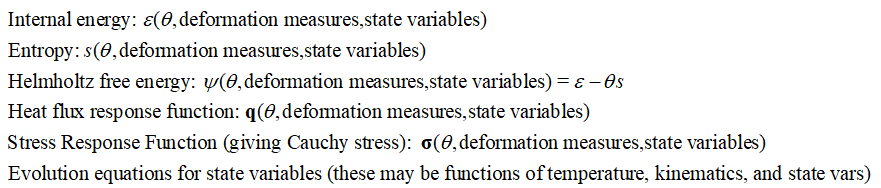
3.1.1 Thermodynamic restrictions

 

Constitutive laws usually start by expressing the specific internal or free energy, specific entropy, and heat flux of a material in terms of the temperature $\theta$, deformation measures characterizing shape changes, and any internal state variables (such as yield stress) that characterize the material state.  These have the general form

 

$\begin{array}{l}\text{Internal energy: }\epsilon (\theta ,\text{deformation measures,state variables)}\\ \text{Entropy: }s(\theta ,\text{deformation measures,state variables)}\\ \text{Helmholtz free energy: }\psi (\theta ,\text{deformation measures,state variables) = }\epsilon -\theta s\\ \text{Heat flux response function: }q(\theta ,\text{deformation measures,state variables)}\\ \text{Stress Response Function (giving Cauchy stress): }\sigma (\theta ,\text{deformation measures,state variables)}\\ \text{Evolution equations for state variables (these may be functions of temperature, kinematics, and state vars)}\end{array}$

 

For a solid with mass density (in the deformed configuration) $\rho$ experiencing a stretch rate $D_{ij}$ and Cauchy stress ${\sigma }_{ij}$, the first and second laws of thermodynamics then require that

$\rho {\left.{\displaystyle \frac{\partial \epsilon }{\partial t}}\right|}_{x=const}={\sigma }_{ij}{D}_{ij}-{\displaystyle \frac{\partial q_i}{\partial y_i}+q}$

${\sigma }_{ij}{D}_{ij}-{\displaystyle \frac{1}{\theta }{q}_i{\displaystyle \frac{\partial \theta }{\partial y_i}-\rho \left({\displaystyle \frac{\partial \psi }{\partial t}+s{\displaystyle \frac{\partial \theta }{\partial t}}}\right)\ge 0}}$

for all possible processes.  The second condition is called the “free energy imbalance.”  It is often convenient to express the condition in terms of other deformation and stress measures. To this end, define:

 

· Mass per unit reference volume ${\rho }_0$ 

 

· Deformation gradient, right Cauchy-Green deformation tensor and Lagrange strain

$F,C=F^{T}F,E=(C-I)/2$

 

· Nominal and material stress $S=J{F}^{-1}\sigma \Sigma =J{F}^{-1}\sigma F^{-T}$

 

· Referential heat flux $Q=J{F}^{-1}q$ 

 

With these definitions, the free energy imbalance condition can be re-written as

$\begin{array}{l}{S}_{ij}{\displaystyle \frac{d{F}_{ji}}{dt}-{\displaystyle \frac{1}{\theta }{Q}_i{\displaystyle \frac{\partial \theta }{\partial x_i}-{\rho }_0\left({\displaystyle \frac{\partial \psi }{\partial t}+s{\displaystyle \frac{\partial \theta }{\partial t}}}\right)\ge 0}}}\\ {\displaystyle \frac{1}{2}{\Sigma }_{ij}{\displaystyle \frac{d{C}_{ij}}{dt}-{\displaystyle \frac{1}{\theta }{Q}_i{\displaystyle \frac{\partial \theta }{\partial x_i}-{\rho }_0\left({\displaystyle \frac{\partial \psi }{\partial t}+s{\displaystyle \frac{\partial \theta }{\partial t}}}\right)\ge 0}}}}\\ {\Sigma }_{ij}{\displaystyle \frac{d{E}_{ij}}{dt}-{\displaystyle \frac{1}{\theta }{Q}_i{\displaystyle \frac{\partial \theta }{\partial x_i}-{\rho }_0\left({\displaystyle \frac{\partial \psi }{\partial t}+s{\displaystyle \frac{\partial \theta }{\partial t}}}\right)\ge 0}}}\end{array}$

You can try deriving these as an exercise.

 

In practice, we usually use only the free energy imbalance law when developing constitutive equations.  The first law can always be satisfied by some appropriate heat flux q. Furthermore, for the majority of problems in solid mechanics, we do not need to model deformation and heat conduction simultaneously (there are exceptions of course, such as high strain rate deformation; thermoelasticity, and so on).   We can assume that the solid is in equilibrium with a surrounding heat bath with constant temperature, and heat flow through a solid is sufficiently rapid to ensure that the temperature remains approximately uniform.  Under these conditions the free energy imbalance condition reduces to

${\sigma }_{ij}{D}_{ij}-\rho {\displaystyle \frac{\partial \psi }{\partial t}\ge 0}$

This expression can be re-written in terms of other stress and deformation measures if need be.  Physically, it states that the rate of work done by stresses must always equal or exceed the rate of change of free energy of the solid. 

 

As a specific example, suppose that we are interested in developing constitutive equations for an elastic solid that is subjected to large deformations (these are called ‘hyperelastic’ materials).  Examples of equations used in practice are listed in Section 3.5.   One way to do this would be to find a scalar function that quantifies the Helmholtz free energy $\psi (C,\theta )$ of our material as a function of the right Cauchy-Green strain tensor C and temperature $\theta$.    The general free energy imbalance condition then requires that

${\displaystyle \frac{1}{2}{\Sigma }_{ij}{\displaystyle \frac{d{C}_{ij}}{dt}-{\displaystyle \frac{1}{\theta }{Q}_i{\displaystyle \frac{\partial \theta }{\partial x_i}-{\rho }_0\left({\displaystyle \frac{\partial \psi }{\partial t}+s{\displaystyle \frac{\partial \theta }{\partial t}}}\right)\ge 0}}}}$

for all possible variations of C and $\theta$.   Taking the time derivative of the free energy and substituting into the free energy imbalance condition gives

$\left({\displaystyle \frac{1}{2}{\Sigma }_{ij}-{\rho }_0{\displaystyle \frac{\partial \psi }{\partial C_{ij}}}}\right){\displaystyle \frac{d{C}_{ij}}{dt}-{\displaystyle \frac{1}{\theta }{Q}_i{\displaystyle \frac{\partial \theta }{\partial x_i}-{\rho }_0\left({\displaystyle \frac{\partial \psi }{\partial \theta }+s}\right){\displaystyle \frac{\partial \theta }{\partial t}\ge 0}}}}$

Since this must hold for all $\partial C_{ij}/\partial t,\partial \theta /\partial x_i,\partial \theta /\partial t$ (with $\theta >0$ ) we conclude that the material stress and entropy must be related to our free energy function by

${\Sigma }_{ij}=2{\rho }_0{\displaystyle \frac{\partial \psi }{\partial C_{ij}}s=-{\displaystyle \frac{\partial \psi }{\partial \theta }}}$

while the heat conduction law must satisfy

$Q_i{\displaystyle \frac{\partial \theta }{\partial x_i}\le 0}$

In Section 3.5, constant temperature versions of this type of constitutive equation are developed by choosing specific functions for the strain energy density $W={\rho }_0\psi$ that can be fit to experiment.  The stress-strain law then follows from the free energy imbalance condition.

 

 

 

3.1.2 Material Frame Indifference (Objectivity):

 

The principle of material frame indifference is two simple ideas: (i) the stress (or strictly speaking the change in stress) in a solid is determined only by the way it changes its shape, and nothing else; and (ii) the constitutive model should predict the correct stress for any mathematical way we choose to describe its motion and deformation.   We can regard the first idea as a consequence of the principle of local action, and it appears to be a reasonable assumption about the way solids behave.   The second is self evident.  Unfortunately, the way we actually test whether a constitutive model satisfies frame indifference involves a rather confusing thought experiment and some complicated mathematics.  As a result, the principle has been questioned and there is a substantial and often confusing literature on the subject (Frewer, 2009, has a nice review). 

 

To test for frame indifference, we need to check that the constitutive law ‘works for any possible mathematical way we choose to describe its motion and deformation.’    In all the constitutive laws discussed in this book, the change in a shape and orientation of a material element is described by the deformation gradient or some other strain measure that can be expressed in terms of this quantity.   So, we need to check that the model works for any conceivable way we might calculate the deformation gradient.   Recall that we calculate the deformation gradient as follows (i) Choose a ‘reference configuration’ for the solid, which assigns each particle in the material a coordinate X.  (ii) Write down the position of each particle after deformation as a function of time $y(X,t)$, and then (iii) Calculate the deformation gradient as $F=\nabla y$ - or if we choose a coordinate system, we can say $F_{ij}=\partial y_i/\partial X_j$.

 

We normally use the initial physical region occupied by the specimen to choose X $–$ so for example if we wanted to calculate the change in length of a vertical tensile bar we would compare it to its initial length $–$ i.e. using a vertical tensile bar as the reference configuration.    But there is no reason why we have to do this.   We could equally well compare its length to that of an undeformed horizontal tensile bar.   This amounts to rotating the ‘reference configuration’ for the bar from a vertical to a horizontal orientation.   In fact, if we are rather strange (e.g. mathematicians), we might even calculate the change in length by comparing it to the initial length of an imaginary undeformed tensile bar that is spinning around in space.   This means we are using a rotating reference configuration.    But as long as we do the calculations correctly, we can still calculate the change in length of the specimen.

 

This is essentially the test we use to check that a constitutive law satisfies the principle of material frame indifference $–$ the goal is to make sure that the constitutive model works for any possible choice of reference configuration that preserves the shape of the solid, including one that rotates in space.   However, since we have to describe more than just a length change the mathematics is a bit more complicated.  

The thought experiment we use for this purpose is illustrated in the figure.  We suppose that the deformation of a solid is observed (and modeled mathematically) by two observers.   The first observer is a normal person, who describes shape changes using the initial configuration of the solid as the reference configuration $–$ this is how we have treated deformation in the rest of this book, to give the deformation mapping a simple physical interpretation.   The second observer is a crazy mathematician, who chooses to use an imaginary reference configuration that has the same shape as the actual initial configuration of the solid, but which rotates and translates through space.  Furthermore, the crazy mathematician chooses to model everything using a coordinate system that rotates and translates with this imaginary reference configuration (this is necessary because the reference configuration has to be time independent).  This might seem a bit disturbing, because this coordinate system is not an inertial frame, but that doesn’t matter $–$ we can use any coordinate system to analyze motion in the actual inertial frame, as long as we transform the vectors in physical space to the rotating frame correctly.  In fact, we do this without thinking when we analyze particle motion using cylindrical polar coordinates: since the polar basis vectors $e_r,e_{\theta }$ rotate with respect to the inertial frame, we use a modified definition of acceleration in the rotating basis, but the formula for acceleration in polar coordinates still describes the acceleration in the inertial frame.   The views of the world with respect to these two observers is shown in the figure: both see a stationary reference configuration with an identical shape.  The rotating observer sees exactly the same deformed solid as the stationary observer, but the whole world appears to be spinning and moving with respect to his or her coordinate system.

 

We discussed how the vectors and tensors that we use to describe motion and deformation of a solid are transformed from the inertial frame (used by the sane observer) to the rotating frame (used by the crazy observer) in Section 2.7. Recall that vectors specifying a particular point in space transform between these frames as

$r^{*}=r_0^{*}(t)+Q(t)(r-r_0)$

where $r$ are three real numbers specifying a point in the inertial frame; $r^{*}$ are the new coordinates of the same point in the rotating frame (these are now three time dependent numbers, reflecting the fact that a fixed point in the inertial frame appears to move in the rotating frame), $r_0$ is an arbitrary point in the inertial frame, $r_0^{*}(t)$ is an arbitrary vector valued function of time t and $Q$ is a time dependent proper orthogonal tensor ( $Q{Q}^T=I$ and $\det (Q)=1$ ).  The coordinates of points in the reference configuration transform as $X^{*}=X$ (because both observers see an identical reference configuration, and we have chosen to put their reference configurations in the same place in their two coordinate systems). 

 

We showed that the coordinates of vectors and tensors we use in continuum mechanics must transform in a predictable way from the inertial frame to the rotating frame as a result of this transformation.  There is a list in Section 2.7.   For example, we found that Cauchy stress tensors and the stretch rate tensors must transform as

${\sigma }^{*}=Q\sigma Q^T{D}^{*}=QD{Q}^T$

(tensors of this kind are called ‘frame indifferent’ or ‘objective’).  Here, ${\sigma }^{*}$ are the numbers that the rotating observer would use to characterize Cauchy stress, while $\sigma$ are the corresponding numbers used by the observer in the inertial frame.  Although they are different, both sets of numbers quantify the force per unit area acting on the same physical element of surface in the solid.  The numbers representing deformation gradient, material stress and Lagrange strain transform as

$F^{*}=QF{\Sigma }^{*}=\Sigma E^{*}=E$

 

Constitutive equations are functions that relates some tensor valued deformation measure(s) to some other tensor valued stress measure.   They are tensor valued functions of one or more tensor valued variable.    There are infinitely many such functions $–$ but the principle of material frame indifference requires that the tensor valued quantity these functions claim to predict must transform correctly under our change of coordinate system and reference configuration.   It is a way to ensure that the material model will predict the same behavior for all possible mathematical descriptions of how the solid changes its shape $–$ even a very strange description in which we use a rotating reference configuration and a rotating coordinate system.

 

So for example a simple linear viscous constitutive law defined (in the inertial frame) by the equation

$\sigma =\eta D+\text{}K\left(\det (F)-1\right)I$

(where $\eta$ and $K$ are constants) is material frame indifferent, because if we use coordinates in the rotated frame it predicts correctly that they are related by

${\sigma }^{*}=\eta D^{*}+\text{}K\left(\det (F^{*})-1\right)I$

To see this, note that $D^{*}=QD{Q}^T,\det (F^{*})\text{}=\det (F),I=QI{Q}^T$, so that substituting and factoring:

$\eta D^{*}+K\left(\det (F^{*})-1\right)I=Q\left\{\eta D+K\left(\det (F)-1\right)I\right\}{Q}^T=Q\sigma Q^T$

which is consistent with the required transformation of Cauchy stress ${\sigma }^{*}=Q\sigma Q^T$ . But a constitutive equation of the form $\sigma =\eta L+(K\det (F)-1)I$ where L denotes the velocity gradient is not material frame indifferent because $L^{*}\ne QL{Q}^T$ (see section 2.7).  Of course, this constitutive equation makes no sense in any case, because $\sigma$ is symmetric and L is not!

 

This does not mean that constitutive equations can only be expressed in terms of frame indifferent tensors, however.   A (rather simple minded) elastic constitutive law that relates material stress to Lagrange strain by the equation

${\Sigma }^{}=cE$

satisfies the principle of material frame indifference, because both material stress and Lagrange strain are invariant under our change of reference frame.

 

Most modern constitutive equations try to describe the underlying microscopic processes that govern its response, and if this is done properly, the law will be frame indifferent.   But some constitutive laws are just curve-fits $–$ some mathematical relationship between a deformation measure and a force measure $–$ and not all possible relationships will transform correctly.  

 

Problems arise most commonly in trying to develop rate forms of constitutive equations, which are intended to relate some measure of strain rate to stress rate.   For example we might try to express a rather dumb elastic constitutive law in rate form as

${\displaystyle \frac{d\sigma }{dt}=cD}$

 This constitutive equation is not material frame indifferent, because we showed in Section 2.7 that D is a frame indifferent tensor but $d\sigma /dt$ is not.  It is not hard to see the cause of this problem $–$ if we consider a stretched tensile specimen that rotates in space, the stresses would clearly change with time, because the principal directions of stress rotate. But the solid is not changing its shape, so the constitutive law says the stress rate should be zero.   The test for ‘frame indifference’ warns us of this inconsistency.

 

There are various fixes for this $–$ the constitutive law can be written in terms of invariant quantities (eg by relating the rate of change of material stress to Lagrange strain rate); they can be derived from physical principles, in which case frame indifferent measures usually emerge naturally from the treatment; or frame indifferent measures of time derivatives can be specially constructed.

 

As a specific example, one way to construct a frame indifferent stress rate is to use the rate of change of stress components with respect to a basis that rotates with the solid (this is what an observer rotating with the material would actually see).  This sounds easy $–$ we just choose some basis vectors $\{m_1,m_2,m_3\}$ with each basis vector parallel to a particular material fiber.  But this doesn’t quite work, because of course the basis vectors won’t generally remain orthogonal under an arbitrary deformation.   So rather than attach $\{m_1,m_2,m_3\}$ to particular material fibers, we simply suppose that they rotate with the average angular velocity of all material fibers passing through a particular point.  This means that

${\displaystyle \frac{d{m}_i}{dt}=W{m}_i}$

where W is the spin tensor.  Now, the time derivative of stress can be written as

${\displaystyle \frac{d\sigma }{dt}={\displaystyle \frac{d}{dt}({\sigma }_{ij}{m}_i\otimes m_j)={\displaystyle \frac{d{\sigma }_{ij}}{dt}{m}_i\otimes m_j+{\sigma }_{ij}W{m}_i\otimes m_j+{\sigma }_{ij}{m}_i\otimes W{m}_j=\stackrel{\nabla }{\sigma }+W\sigma -\sigma W}}}$

Here, the first term on the right hand side can be interpreted as the stress rate seen by an observer who rotates with the material; while the second and third are the additional rate of change of stress caused by the rotation of the material.  The first term on the right hand side is called the Jaumann stress rate.  It is defined as

$\stackrel{\nabla }{\sigma }={\displaystyle \frac{d\sigma }{dt}-W\sigma +\sigma W}$

 We showed in Section 2.7 that $\stackrel{\nabla }{\sigma }$ is frame indifferent. Many constitutive equations assume that material stretch rate is proportional to this special stress rate.  For example, we could write

$\stackrel{\nabla }{\sigma }=\tilde{C}D$

Provided that $\tilde{C}$ is a frame indifferent fourth-order tensor, this constitutive equation would be frame indifferent.

 

Hopefully this discussion has convinced you that the principle of material frame indifference is a mathematical consequence of the way we describe stresses and shape changes in a solid, and is necessary to ensure that solid mechanics is self-consistent. The various objections to the principle that can be found in the literature arise because there is a more restrictive (and hence controversial) version of the principle that asserts that a material in a rotating frame (e.g. when tested in a centrifuge) must have the same stress-strain behavior as a stationary specimen.   This happens to be true for virtually all constitutive equations that are in common use, but it is better to regard this as a prediction resulting from the principle of material frame indifference and the particular choice of strain measures in these models, rather than a general assumption about the way materials must behave.   It is perfectly possible to construct continuum theories of solids in which a change in orientation or a nonzero angular velocity will influence the stresses in the material, while satisfying the version of frame indifference described in this book.    These theories need to make use of frame indifferent measures of the angular velocity of the solid (which would depend on the spin $\Omega$ of the observer relative to the inertial frame). They may also need to use more elaborate descriptions of deformation and internal forces than the constitutive equations discussed in this chapter (e.g. strain measures involving higher order derivatives of the deformation mapping, or force measures quantifying internal moments). 

 

 In closing, however, it is worth pointing out that the solid mechanicians concept of a ‘shape change’ (which leads to the concept of a reference configuration and hence frame indifference) cannot be applied to all materials. For example, suppose we try to apply the conventional view of a solid to model a 2-phase gas that contains atoms of species A and B.    At any instant, we can certainly define a ‘material element’ in the sense of solid mechanics by choosing a reasonably large tetrahedron connecting some suitable subset of 4 atoms in the gas.  We can then define quantities such as ‘density,’  ‘concentration,’  ‘internal material surface’ and so on, and describe the behavior of this volume using the ideas in this book.  We can use this approach to model sound wave propagation through the gas, for example. But this view of a gas becomes problematic if we recall that we also use some separate laws to describe how A and B mix.   For example, if we start with a container in which A and B have a non-uniform concentration, the concentration will gradually evolve to become uniform (assuming the atoms have the same mass or the container is in zero gravity!).  We think of this process as ‘diffusion’ and model it with Fick’s law. But if atoms can diffuse, it becomes difficult to define a ‘material element’ in the sense of solid mechanics, because atoms would slowly cross any imaginary surfaces we place inside the gas. In reality there is no easy way to distinguish between ‘diffusion’ and ‘deformation’ at the atomic scale.   Both are just motion of atoms as a result of interactions with their neighbors $–$ they just occur at different time scales.  Of course, we would not idealize a gas as a solid in most calculations.  Many theories of gas flow do not use concepts such as a ‘material volume’ and ‘material surface;’ they also do not attempt to describe the undeformed ‘shape’ of a gas.   Instead, they quantify stresses by tractions acting on fixed spatial surfaces, and use stress measures that include contributions from the momentum transport through these surfaces. They also use concepts such as ‘partial stresses’ to quantify the stresses associated with different phases in the gas.   These theories have to be ‘frame indifferent’ in some sense, but the solid mechanics version of frame indifference does not apply.  This may sound appealing to those who question the principle of material frame indifference, but theories that describe gas or fluid flow are difficult to apply to solids, because they cannot easily describe the tendency of a solid to return to a preferred shape when it is unloaded. They do not even have a clear description of how external forces act on a physical element of material.  Perhaps in future a unified continuum theory will emerge that does not distinguish between gases, fluids and solids.   In the meantime, we have to remember that all our models are approximations, and apply them only when these approximations are valid.

 

 

 

3.1.3 Drucker Stability 

 

For most practical applications, the constitutive equation must satisfy a condition known as the Drucker stability criterion, which can be expressed as follows.  Consider a deformable solid, subjected to boundary tractions $t_i$, which induce some displacement field $u_i$, as shown in the figure. Suppose that the tractions are increased to $t_i+\Delta t_i$, resulting in an additional displacement $\Delta u_i$. The material is said to be stable in the sense of Drucker if the work done by the tractions $\Delta t_i$ through the displacements $\Delta u_i$ is positive or zero for all $\Delta t_i$:

$\Delta W={\displaystyle \int \left\{{\displaystyle \underset{A}{\int }\Delta t_i{\displaystyle \frac{d\Delta u_i}{dt}}}\right\}}dt\ge 0$

You can show that this condition is satisfied as long as the stress-strain relation obeys

$\Delta {\tau }_{ij}\Delta {\epsilon }_{ij}\ge 0$

where $\Delta {\tau }_{ij}$ is the change in Kirchhoff stress, and $\Delta {\epsilon }_{ij}=(\partial \Delta u_i/\partial x_j+\partial \Delta u_j/\partial x_i)$ is an increment in strain resulting from an infinitesimal change in displacement $\Delta u_i$.

 

This is not a thermodynamic law (the work done by the change in tractions is not a physically meaningful quantity), and there is nothing to say that real materials have to satisfy Drucker stability. In fact, many materials show clear signs that they are not stable in the sense of Drucker.   However, if you try to solve a boundary value problem for a material that violates the Drucker stability criterion, you are likely to run into trouble.  The problem will probably not have a unique solution, and in addition you are likely to find that smooth curves on the undeformed solid develop kinks (and may not even be continuous) after the solid is deformed.  This kind of deformation violates one of the fundamental assumptions underlying continuum constitutive equations. 

 

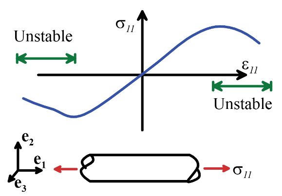A simple example of a stress-strain curve for material that is not stable in the sense of Drucker is shown in the figure. The stability criterion is violated wherever the stress decreases with strain in tension, or increases with strain in compression. For the former we see that $\Delta {\sigma }_{11}<0$, while $\Delta {\epsilon }_{11}>0$; for the latter $\Delta {\sigma }_{11}>0$, while $\Delta {\epsilon }_{11}<0$.

 

In the following chapter, we outline constitutive laws that were developed to approximate the behavior of a wide range of materials, including polycrystalline metals and non-metals; elastomers; polymers; biological tissue; soils; and metal single crystals.  A few additional material models, which account for material failure, are described in Chapter 9.