3.2 Linear elastic
material behavior
Linear elastic stress-strain laws are
used to describe the behavior of materials that experience small, reversible
strains when subjected to modest stress. You are probably familiar with the
behavior of a linear elastic material from introductory materials courses. Their
main features are reviewed briefly below.
3.2.1 Isotropic, linear elastic material behavior
If you conduct a uniaxial tensile test on almost any
material, and keep the stress levels sufficiently low, you will observe the
following behavior:
· The specimen deforms reversibly: if you remove the loads, the solid returns to
its original shape.
· The strain in the specimen depends only on the stress
applied to it it doesn’t depend on the rate of loading, or
the history of loading.
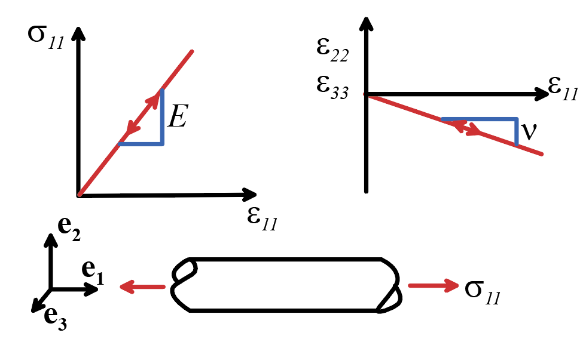
· For most materials, the stress is a linear function of
strain, as shown in the figure. Because the strains are small, this is true
whatever stress measure is adopted (Cauchy stress or nominal stress), and is
true whatever strain measure is adopted (Lagrange strain or infinitesimal
strain).
·  For most, but not
all, materials, the material has no characteristic orientation. Thus, if you cut a tensile specimen out of a block
of material, as shown in the figure, the stressstrain curve will be
independent of the orientation of the specimen relative to the block of material. Such materials are said to be isotropic.
For most, but not
all, materials, the material has no characteristic orientation. Thus, if you cut a tensile specimen out of a block
of material, as shown in the figure, the stressstrain curve will be
independent of the orientation of the specimen relative to the block of material. Such materials are said to be isotropic.
· If you heat a
specimen of the material, increasing its temperature uniformly, it will
generally change its shape slightly. If
the material is isotropic (no preferred material orientation) and homogeneous,
then the specimen will simply increase in size, without shape change.
3.2.2 Stressstrain relations for isotropic, linear elastic
materials. Young’s Modulus, Poissons ratio and the Thermal Expansion
Coefficient.
Before writing down
stressstrain relations, we
need to decide what strain and stress measures we want to use. Because the model only works for small shape
changes
· Deformation is characterized using the infinitesimal
strain tensor defined in Section 2.2.10. This is convenient for calculations, but has
the disadvantage that linear elastic constitutive equations can
only be used if the solid experiences small rotations, as well as small shape
changes.
· All stress measures are taken to be equal. We can use the Cauchy stress as the stress measure.
You probably already
know the stressstrain relations for
an isotropic, linear elastic solid. They
are repeated below for convenience.

Here, E and are Young’s modulus and Poisson’s ratio, is the coefficient of thermal expansion, and is the increase in temperature of the
solid. The remaining relations can be
deduced from the fact that both and are symmetric.
The inverse relationship can be
expressed as

HEALTH WARNING: Note
the factor of 2 in the strain vector.
Most texts, and most finite element codes use this factor of two, but
not all. In addition, shear strains and
stresses are often listed in a different order in the strain and stress
vectors. For isotropic materials this
makes no difference, but you need to be careful when listing material constants
for anisotropic materials.
We can write this expression in a
much more convenient form using index notation.
Verify for yourself that the matrix expression above is equivalent to
The inverse relation is
The stress-strain
relations are often expressed using the elastic
modulus tensor or the elastic
compliance tensor as
In terms of elastic constants, and are
3.2.3 Reduced stress-strain equations for plane deformation of isotropic
solids
For plane strain or plane stress deformations, some strain or stress components are
always zero (by definition) so the stress-strain laws can be simplified.
· For a plane strain
deformation . The stress strain laws are therefore
In index notation
where Greek subscripts can have values 1 or 2.
· For a plane stress deformation , and the
stres-strain relations are
3.2.4 Representative values for density, and elastic
constants of isotropic solids
The table below shows representative elastic constants for a range of different
materials. The data are partly from Jones and Ashby (2019), and partly from manufacturers
data sheets.
Note the units
values of E
are given in ; the G stands for Giga, and is short
for .
The units for density are in - that’s Mega grams. One mega gram is 1000 kg.

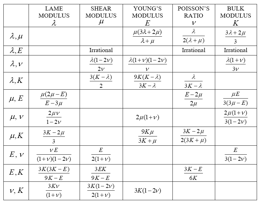
3.2.5 Other Elastic Constants bulk, shear and Lame modulus.
Young’s modulus and
Poisson’s ratio are the most common properties used to characterize elastic
solids, but other measures are also used.
For example, we define the shear
modulus, bulk modulus and Lame
modulus of an elastic solid as follows:
The table below relates all the possible combinations of moduli to all other
possible combinations. Enjoy!
3.2.6 Physical interpretation of elastic constants for
isotropic solids
It is important to have a feel for the
physical significance of the various elastic constants. They can be interpreted as follows
· Young’s modulus E is the slope of the stressstrain curve in uniaxial
tension. It has dimensions of stress ( ) and is usually large for steel, . You can think of E as a measure of the stiffness of the
solid. The larger the value of E, the
stiffer the solid. For a stable
material, the Young’s modulus must satisfy E>0.
· Poisson’s ratio is the ratio of lateral to longitudinal strain
in uniaxial tensile stress. It is dimensionless and typically ranges from 0.20.49, and is around 0.3 for most
metals. For a stable material, Poisson’s
ratio is in the range . It is a measure of the
compressibility of the solid. If , the solid is incompressible its volume remains constant, no matter how it
is deformed. If , then stretching a specimen causes
no lateral contraction. Some bizarre
materials have -- if
you stretch a round bar of such a material, the bar increases in diameter!!
· Thermal expansion coefficient quantifies the change in volume of a material if it is
heated in the absence of stress. It has
dimensions of (degrees Kelvin)-1 and is usually very small. For steel,
· The bulk modulus
quantifies the resistance of the solid to volume changes. It has a large value (usually bigger than E).
· The shear modulus
quantifies its resistance to volume preserving shear deformations. Its value is usually somewhat smaller than E.
3.2.7 Strain Energy Density for Isotropic Solids
The following observations are the basis for defining the
strain energy density of an elastic material
· If you deform a block of material,
you do work on it (or, in some cases, it may do work on you…)
· In an elastic material, the work done
during loading is stored as recoverable strain energy in the solid. If you unload the material, the specimen does
work on you, and when it reaches its initial configuration you come out even.
· The work done to deform a specimen
depends only on the state of strain at the end of the test. It is independent of the history of
loading.
Based on these observations, we
define the strain energy density of
a solid as the work done per unit volume to deform a material from a stress
free reference state to a loaded state.
To write down an expression for the
strain energy density, it is convenient to separate the strain into two parts
where, for an isotropic solid,
represents the strain due to thermal expansion (known as
thermal strain), and
is the strain due to mechanical loading (known as elastic
strain).
Work is done on the specimen only
during mechanical loading. It is
straightforward to show that the strain energy density is
You can also re-write this as
Observe that
3.2.8 Stress-strain relation for a
general anisotropic linear elastic material the elastic stiffness and compliance
tensors
The simple isotropic model described
in the preceding section is unable to describe the response of some materials
accurately, even though the material may deform elastically. This is because some materials do have a
characteristic orientation. For example,
in a block of wood, the grain is oriented in a particular direction in the
specimen. The block will be stiffer if
it is loaded parallel to the grain than if it is loaded perpendicular to the
grain. The same observation applies to fiber
reinforced composite materials. Generally, single crystal specimens of a
material will also be anisotropic this is important when modeling stress effects
in small structures such as microelectronic circuits. Even polycrystalline
metals may be anisotropic, because a preferred texture may form in the specimen
during processing.
A more general stressstrain relation is needed to describe
anisotropic solids.
The most general linear stressstrain relation has the form
Here, is a fourth order tensor (horrors!), known as
the elastic stiffness tensor, and is the thermal expansion coefficient tensor.
The stress strain relation is invertible:
where is known as the elastic compliance tensor
At first sight it appears that the
stiffness tensor has 81 components.
Imagine having to measure and keep track of 81 material properties! Fortunately, must have the following symmetries
This reduces the number of material
constants to 21. The compliance tensor has the same symmetries as .
To see the origin of the symmetries
of , note that
· The stress tensor is symmetric, which
is only possible if
· If a strain energy density exists for
the material, the elastic stiffness tensor must satisfy
· The previous two symmetries imply , since and .
To see that , note that by definition
and recall further that the stress is the derivative of the
strain energy density with respect to strain
Combining these,
Now, note that
so that
These symmetries allow us to write the stress-strain
relations in a more compact matrix form as
where , etc are the elastic stiffnesses of the material. The inverse has the form
where , etc are the elastic compliances of the material.
To satisfy Drucker stability, the eigenvalues
of the elastic stiffness and compliance matrices must all be greater than zero.
HEALTH WARNING: The shear strain and shear stress components are not always listed in the
order given when defining the elastic and compliance matrices. The conventions used here are common and are
particularly convenient in analytical calculations involving anisotropic
solids. But many sources use other
conventions. Be careful to enter
material data in the correct order when specifying properties for anisotropic
solids.
3.2.9 Physical Interpretation of the
Anisotropic Elastic Constants.
 It is easiest to interpret , rather than .
Imagine applying a uniaxial stress, say , to an anisotropic specimen. In general, this would induce both
extensional and shear deformation in the solid, as shown in the figure.
It is easiest to interpret , rather than .
Imagine applying a uniaxial stress, say , to an anisotropic specimen. In general, this would induce both
extensional and shear deformation in the solid, as shown in the figure.
The strain induced
by the uniaxial stress would be
All the constants
have dimensions . The constant looks like a uniaxial compliance, (like ), while the
ratios are generalized versions of Poisson’s ratio:
they quantify the lateral contraction of a uniaxial tensile specimen. The shear terms are new in an isotropic material, no shear strain is
induced by uniaxial tension.
3.2.10 Strain energy density for anisotropic, linear elastic solids
The strain energy density of an
anisotropic material is
3.2.11 Basis change formulas for anisotropic elastic constants
The material constants or for a particular material are usually
specified in a basis with coordinate axes aligned with particular symmetry
planes (if any) in the material. When
solving problems involving anisotropic materials it is frequently necessary to
transform these values to a coordinate system that is oriented in some
convenient way relative to the boundaries of the solid. Since is a fourth rank tensor, the basis change
formulas are highly tedious, unfortunately.
 Suppose that the components of the
stiffness tensor are given in a basis , and we wish to determine its
components in a second basis, , as shown in the figure. We define the usual transformation tensor with components , or in matrix form
Suppose that the components of the
stiffness tensor are given in a basis , and we wish to determine its
components in a second basis, , as shown in the figure. We define the usual transformation tensor with components , or in matrix form
This is an orthogonal matrix
satisfying . In practice, the matrix can be
computed in terms of the angles between the basis vectors. It is
straightforward to show that stress, strain, thermal expansion and elasticity
tensors transform as
The basis change formula for the elasticity tensor in matrix
form can be expressed as
where the basis change matrix K is computed as
and the modulo function satisfies
Although these expressions look
cumbersome they are quite easy to code in a computer program.
The basis change for the compliance tensor follows as
where
The proof of these expressions is
merely tiresome algebra and will not be given here. Ting (1996) has a nice clear discussion.
For the particular case of rotation
through an angle with right hand screw convention about the axes, respectively, the rotation matrix for
the elasticity tensor reduces to
Rotation about
Rotation about
Rotation about
where . The inverse matrix can be obtained simply by changing the sign of
the angle in each rotation matrix. Applying the three rotations successively can
produce an arbitrary orientation change.
For an isotropic material, the
elastic stress-strain relations, the elasticity matrices and thermal expansion
coefficient are unaffected by basis changes.
3.2.12 The effect of material symmetry on stress-strain relations for
anisotropic materials
A general anisotropic solid has 21
independent elastic constants. Note that, in general, tensile stress may induce
shear strain, and shear stress may cause extension.

If a material has a symmetry plane,
then applying stress normal or parallel to this plane, as shown in the figure, induces
only extension in direction normal and parallel to the plane.
For example, suppose the material
contains a single symmetry plane, and let be normal to this plane. Then the components
of the elastic stiffnes matrix
Or equivalently
(symmetrical terms
also vanish, of course). This leaves 13 independent constants.
Similar restrictions on the thermal
expansion coefficient can be determined using symmetry conditions. Details are left as an exercise.
In the following sections, we list
the stress-strain relations for anisotropic materials with various numbers of
symmetry planes.
3.2.13 Stress-strain relations for linear elastic orthotropic materials
 An orthotropic material has three
mutually perpendicular symmetry planes. This type of material has 9 independent
material constants. With basis vectors
perpendicular to the symmetry planes, as shown in the figure, the
elastic stiffness matrix has the form
An orthotropic material has three
mutually perpendicular symmetry planes. This type of material has 9 independent
material constants. With basis vectors
perpendicular to the symmetry planes, as shown in the figure, the
elastic stiffness matrix has the form
This relationship is sometimes
expressed in inverse form, in terms of generalized Young’s moduli and Poisson’s
ratios (which have the same significance as Young’s modulus and Poisson’s ratio
for uniaxial loading along the three basis vectors) as follows
Here the generalized Poisson’s ratios
are not symmetric but instead satisfy (no sums). This ensures that the stiffness
matrix is symmetric.
The engineering constants are related to the components of
the compliance tensor by
or in inverse form
For an
orthotropic material thermal expansion cannot induce shear (in this basis) but
the expansion in the three directions need not be equal. Consequently the thermal expansion
coefficient tensor has the form
3.2.14
Stress-strain relations for linear elastic Transversely Isotropic Material
A special
case of an orthotropic solid is one that contains a plane of isotropy (this
implies that the solid can be rotated with respect to the loading direction
about one axis without measurable effect on the solid’s response). Choose perpendicular to this symmetry plane. Then, transverse isotropy requires that , , , , so that
the stiffness matrix has the form

The
engineering constants must satisfy
and the compliance matrix has the
form
where .
As before the Poisson’s ratios are not symmetric, but satisfy
The engineering constants and
stiffnesses are related by
For this material the two thermal
expansion coefficients in the symmetry plane must be equal, so the thermal
expansion coefficient tensor has the form
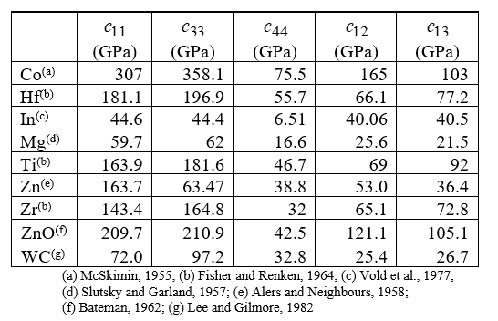
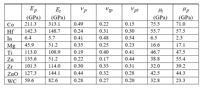
3.2.15 Representative values for elastic
constants of transversely isotropic hexagonal close packed crystals
Hexagonal
close-packed crystals are an example of transversely isotropic materials. The axis must be taken to be perpendicular to the
basal (0001) plane of the crystal, as shown in the figure. Since the plane perpendicular to is isotropic the orientation of and is arbitrary.

A table of
values of stiffnesses for a few hexagonal materials is listed in the table
below
The engineering constants can be
calculated and are listed in the table below
3.2.16 Linear elastic stress-strain relations for cubic materials
A huge
number of materials have cubic symmetry all the FCC and BCC metals, for example. The constitutive law for such a material is
particularly simple, and can be parameterized by only 3 material
constants. Pick basis vectors
perpendicular to the symmetry planes, as shown in Figure 3.12. <Figure 3.12 near here>

Then
or in terms of engineering constants
This is
virtually identical to the constitutive law for an isotropic solid, except that
the shear modulus is not related to the Poisson’s ratio and
Young’s modulus through the usual relation given in Section 3.1.6. In fact, the ratio
provides a convenient measure of
anisotropy. For the material is isotropic.
The thermal expansion coefficient
matrix must be isotropic for materials with cubic symmetry.
The relationships between the
elastic constants are
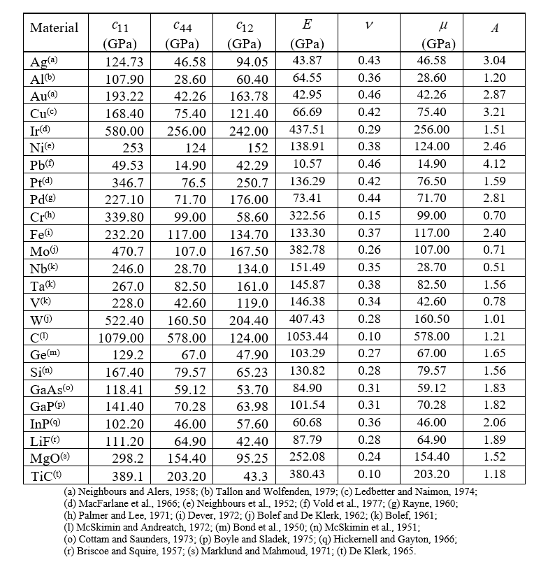
3.2.17 Representative values for elastic properties of cubic crystals and
compounds
The table below lists values of elastic constants for various cubic crystals and
compounds. The elastic constants were calculated using the formulas in the
preceding section.