3.5 Hyperelasticity - time independent behavior of rubbers and foams subjected to large strains

 

Hyperelastic constitutive laws are used to model materials that respond elastically when subjected to very large strains. They account both for nonlinear material behavior and large shape changes.  The main applications of the theory are (i) to model the rubbery behavior of a polymeric material, and (ii) to model polymeric foams that can be subjected to large reversible shape changes (e.g. a sponge). 

 

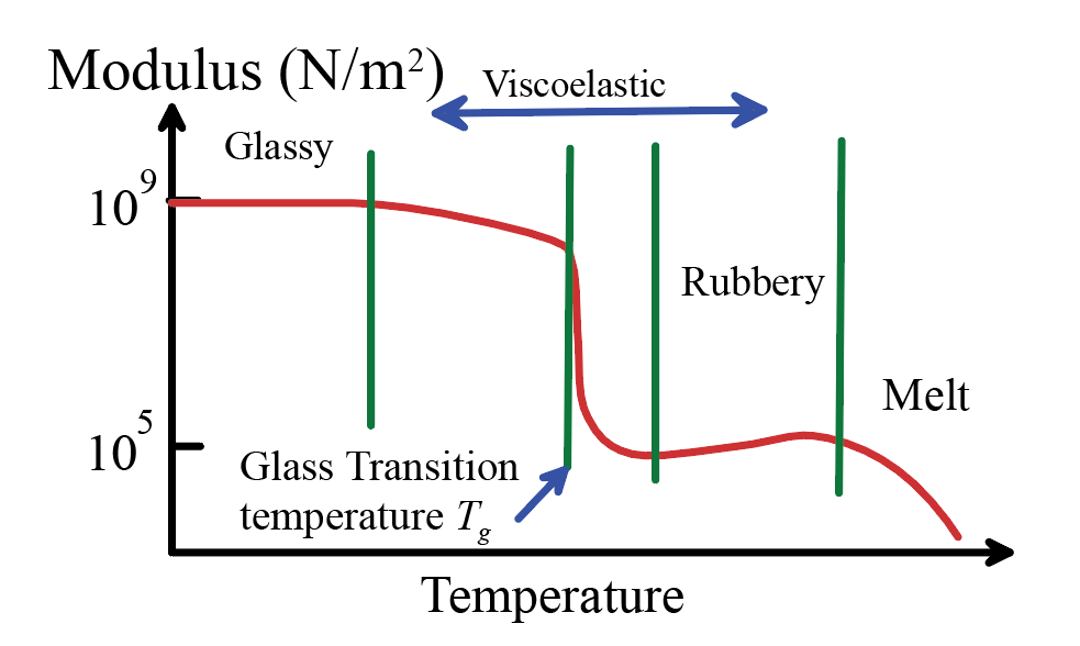
In general, the response of a typical polymer is strongly dependent on temperature, strain history and loading rate.  The behavior will be described in more detail in the next section, where we present the theory of viscoelasticity.  For now, we note that polymers have various regimes of mechanical behavior, referred to as ‘glassy,’ ‘viscoelastic’ and ‘rubbery.’   The various regimes can be identified for a particular polymer by applying a sinusoidal variation of shear stress to the solid and measuring the resulting shear strain amplitude.  A typical result is illustrated in the figure, which shows the apparent shear modulus (ratio of stress amplitude to strain amplitude) as a function of temperature.

 

At a critical temperature known as the glass transition temperature, a polymeric material undergoes a dramatic change in mechanical response.  Below this temperature, it behaves like a glass, with a stiff response. Near the glass transition temperature, the stress depends strongly on the strain rate.  At the glass transition temperature, there is a dramatic drop in modulus.  Above this temperature, there is a regime where the polymer shows ‘rubbery’ behavior - the response is elastic; the stress does not depend strongly on strain rate or strain history, and the modulus increases with temperature.  All polymers show these general trends, but the extent of each regime, and the detailed behavior within each regime, depend on the solid’s molecular structure.  Heavily cross-linked polymers (elastomers) are the most likely to show ideal rubbery behavior.   Hyperelastic constitutive laws are intended to approximate this behavior.

 

 

Features of the behavior of a solid rubber:

 

1. The material is close to ideally elastic. i.e. (i) when deformed at constant temperature or adiabatically, stress is a function only of current strain and independent of history or rate of loading, (ii) the behavior is reversible: no net work is done on the solid when subjected to a closed cycle of strain under adiabatic or isothermal conditions.

 

2. The material strongly resists volume changes.  The bulk modulus (the ratio of volume change to hydrostatic component of stress) is comparable to that of metals or covalently bonded solids;

 

3. The material is very compliant in shear $–$ shear modulus is of the order of ${10}^{-5}$ times that of most metals;

 

4. The material is isotropic $–$ its stress-strain response is independent of material orientation.

 

5. The shear modulus is temperature dependent: the material becomes stiffer as it is heated, in sharp contrast to metals;

 

6. When stretched, the material gives off heat.

 

 

Polymeric foams (e.g. a sponge) share some of these properties:

 

1. They are close to reversible, and show little rate or history dependence.

 

2. In contrast to rubbers, most foams are highly compressible $–$ bulk and shear moduli are comparable.

 

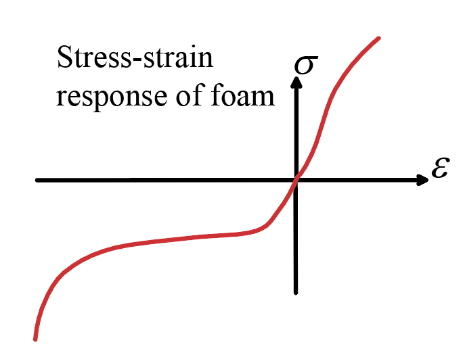
3. Foams have a complicated true stress-true strain response, generally resembling sketch in the figure. The finite strain response of the foam in compression is quite different to that in tension, because of buckling in the cell walls.

 

4. Foams can be anisotropic, depending on their cell structure.   Foams with a random cell structure are isotropic. 

 

The literature on stress-strain relations for finite elasticity can be hard to follow, partly because nearly every paper uses a different notation, and partly because there are many different ways to write down the same stress-strain law.   You should find that most of the published literature is consistent with the framework given below $–$ but it may take some work to show the equivalence.

 

 

All hyperelastic models are constructed as follows:

 

1. Define the stress-strain relation for the solid by specifying its strain energy density W (which is related to the Helmholtz free energy of the solid by $W={\rho }_0\psi$, where ${\rho }_0$ is the mass per unit reference volume)   as a function of the deformation gradient tensor (or some strain measure derived from the deformation gradient): W=W(F).    This ensures that the material is perfectly elastic, and also means that we only need to work with a scalar function.  The general form of the strain energy density is guided by experiment; and the formula for strain energy density always contains material properties that can be adjusted to describe a particular material.

 

2. The undeformed material is often assumed to be isotropic $–$ i.e the behavior of the material is independent of the initial orientation of the material with respect to the loading.  If the strain energy density is a function of the Left Cauchy-Green deformation tensor $B=F{F}^T$ the constitutive equation is automatically isotropic.  To see this, note that if we subject the solid to a rigid rotation R before applying the deformation F we find that $B=FR{(FR)}^T$  so B is unchanged by changing the orientation of the specimen.  But if B is used as the deformation measure, then the strain energy must be a function of the invariants of B to ensure that the constitutive equation is frame indifferent (see Sect 2.7 and 3.1).  This is because under a change of reference frame represented by an orthogonal tensor Q the components of B change to $B^{*}=QB{Q}^T$, but the strain energy must be independent of Q to satisfy frame indifference.  The invariants of $B^{*}$ and $B$ are equal.

 

3. For an anisotropic constitutive equation we can make the strain energy density a function of the Right Cauchy-Green tensor $C=F^{T}F$.   This is automatically frame indifferent because $C^{*}=C$ under a change of reference frame.   But under a rotation R before deformation a deformation F the Cauchy Green tensor is $C=R^T{F}^{T}FR$.  Unlike B, it is not invariant to the orientation of the specimen.

 

4. Formulas for stress in terms of strain are calculated by differentiating the strain energy density as outlined below.

 

 

 

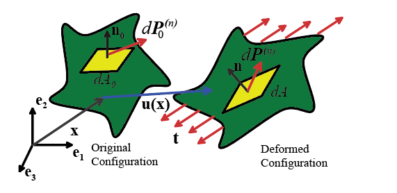
3.5.1 Deformation Measures used in finite elasticity

 

Suppose that a solid is subjected to a displacement field $u_i(x_k)$, as shown in the figure. Define

 

· The deformation gradient and its Jacobian

$F_{ij}={\delta }_{ij}+{\displaystyle \frac{\partial u_i}{\partial x_j}}$       $J=\det (F)$

 

· The Left and Right Cauchy-Green deformation tensors

$B=F{F}^{T}C=F^{T}F{B}_{ij}=F_{ik}{F}_{jk}{C}_{ij}=F_{ki}{F}_{kj}$

 

· Invariants of B (these are the conventional definitions)

$\begin{array}{l}{I}_1=\text{trace}(B)=B_{kk}\\ I_2={\displaystyle \frac{1}{2}\left(I_1^2-B\cdot \cdot B\right)={\displaystyle \frac{1}{2}\left(I_1^2-B_{ik}{B}_{ki}\right)}}\\ I_3=\det B=J^2\end{array}$

 

· An alternative set of invariants of B (more convenient for models of nearly incompressible materials $–$ note that ${\overline{I}}_1,{\overline{I}}_2$ remain constant under a pure volume change)

$\begin{array}{l}{\overline{I}}_1={\displaystyle \frac{I_1}{J^{2/3}}\text{=}{\displaystyle \frac{B_{kk}}{J^{2/3}}}}\\ {\overline{I}}_2={\displaystyle \frac{I_2}{J^{4/3}}={\displaystyle \frac{1}{2}\left({\overline{I}}_1^2-{\displaystyle \frac{B\cdot \cdot B}{J^{4/3}}}\right)={\displaystyle \frac{1}{2}\left({\overline{I}}_1^2-{\displaystyle \frac{B_{ik}{B}_{ki}}{J^{4/3}}}\right)}}}\\ J=\sqrt{\det B}\end{array}$

 

· Principal stretches and principal stretch directions, specified as follows

1. Let $e_1,e_2,e_3$ denote the three eigenvalues of B.  The principal stretches are

${\lambda }_1=\sqrt{e_1},{\lambda }_2=\sqrt{e_2},{\lambda }_3=\sqrt{e_3}$

2. Let $b_1,b_2,b_3$ denote three, mutually perpendicular unit eigenvectors of B. These define the principal stretch directions.  (Note: since B is symmetric its eigenvectors are automatically mutually perpendicular as long as no two eigenvalues are the same.  If two, or all three eigenvalues are the same, the eignevectors are not uniquely defined $–$ in this case any convenient mutually perpendicular set of eigenvectors can be used).

3. Recall that B can be expressed in terms of its eigenvectors and eigenvalues as

$B={\lambda }_1^2{b}^{(1)}\otimes b^{(1)}+{\lambda }_2^2{b}^{(2)}\otimes b^{(2)}+{\lambda }_3^2{b}^{(3)}\otimes b^{(3)}$

 

 

 

3.5.2 Stress Measures used in finite elasticity

 

Usually stress-strain laws are given as equations relating Cauchy stress (`true’ stress) ${\sigma }_{ij}$ to left Cauchy-Green deformation tensor.  For some computations it may be more convenient to use other stress measures.  They are defined below, for convenience.

 

· The Cauchy (“true”) stress represents the force per unit deformed area in the solid and is defined by

$n_i{\sigma }_{ij}=\underset{dA\to 0}{Lim}{\displaystyle \frac{d{P}_j^{(n)}}{dA}}$

 

· Kirchhoff stress  $\tau =J\sigma {\tau }_{ij}=J{\sigma }_{ij}$

 

· Nominal (First Piola-Kirchhoff) stress  $S=J{F}^{-1}\sigma S_{ij}=J{F}_{ik}^{-1}{\sigma }_{kj}$

 

· Material (Second Piola-Kirchhoff) stress  $\Sigma =J{F}^{-1}\sigma F^{-T}{\Sigma }_{ij}=J{F}_{ik}^{-1}{\sigma }_{kl}{F}_{jl}^{-1}$

 

 

 

 

3.5.3 Calculating stress-strain relations from the strain energy density

 

The constitutive law for an isotropic hyperelastic material is defined by an equation relating the strain energy density of the material to the deformation gradient, or, for an isotropic solid, to the three invariants of the strain tensor

$W(F)=U(I_1,I_2,I_3)=\overline{U}({\overline{I}}_1,{\overline{I}}_2,J)=\tilde{U}({\lambda }_1,{\lambda }_2,{\lambda }_3)$

The stress-strain law must then be deduced by differentiating the strain energy density.   This can involve some tedious algebra.  Formulas are listed below for the stress-strain relations for each choice of strain invariant.  The results are derived below

 

 

· Strain energy density in terms of $F_{ij}$

${\sigma }_{ij}={\displaystyle \frac{1}{J}{F}_{ik}{\displaystyle \frac{\partial W}{\partial F_{jk}}}}$

 

· Strain energy density in terms of $C_{ij}$

${\sigma }_{ij}={\displaystyle \frac{2}{J}{F}_{ik}{\displaystyle \frac{\partial W}{\partial C_{kl}}{F}_{jl}}}$

 

· Strain energy density in terms of $I_1,I_2,I_3$

${\sigma }_{ij}={\displaystyle \frac{2}{\sqrt{I_3}}\left[\left({\displaystyle \frac{\partial U}{\partial I_1}+I_1{\displaystyle \frac{\partial U}{\partial I_2}}}\right)B_{ij}-{\displaystyle \frac{\partial U}{\partial I_2}{B}_{ik}{B}_{kj}}\right]+2\sqrt{I_3}{\displaystyle \frac{\partial U}{\partial I_3}{\delta }_{ij}}}$

 

· Strain energy density in terms of ${\overline{I}}_1,{\overline{I}}_2,J$

${\sigma }_{ij}={\displaystyle \frac{2}{J}\left[{\displaystyle \frac{1}{J^{2/3}}\left({\displaystyle \frac{\partial \overline{U}}{\partial {\overline{I}}_1}+{\overline{I}}_1{\displaystyle \frac{\partial \overline{U}}{\partial {\overline{I}}_2}}}\right)B_{ij}-\left({\overline{I}}_1{\displaystyle \frac{\partial \overline{U}}{\partial {\overline{I}}_1}+2{\overline{I}}_2{\displaystyle \frac{\partial \overline{U}}{\partial {\overline{I}}_2}}}\right){\displaystyle \frac{{\delta }_{ij}}{3}-{\displaystyle \frac{1}{J^{4/3}}{\displaystyle \frac{\partial \overline{U}}{\partial {\overline{I}}_2}{B}_{ik}{B}_{kj}}}}}\right]+{\displaystyle \frac{\partial \overline{U}}{\partial J}{\delta }_{ij}}}$

 

· Strain energy density in terms of ${\lambda }_1,{\lambda }_2,{\lambda }_3$

${\sigma }_{ij}={\displaystyle \frac{{\lambda }_1}{{\lambda }_1{\lambda }_2{\lambda }_3}{\displaystyle \frac{\partial \tilde{U}}{\partial {\lambda }_1}{b}_i^{(1)}{b}_j^{(1)}+{\displaystyle \frac{{\lambda }_2}{{\lambda }_1{\lambda }_2{\lambda }_3}{\displaystyle \frac{\partial \tilde{U}}{\partial {\lambda }_2}{b}_i^{(2)}{b}_j^{(2)}+{\displaystyle \frac{{\lambda }_3}{{\lambda }_1{\lambda }_2{\lambda }_3}{\displaystyle \frac{\partial \tilde{U}}{\partial {\lambda }_3}{b}_i^{(3)}{b}_j^{(3)}}}}}}}$

 

 

 

Derivations:   We start by deriving the general formula for stress in terms of $W(F)$:

 

1. Note that, by definition, if the solid is subjected to some history of strain, the rate of change of the strain energy density W (F)  must equal the rate of mechanical work done on the material per unit reference volume.

 

2. Recall that the rate of work done per unit undeformed volume by body forces and surface tractions is expressed in terms of the nominal stress $S_{ij}$ as $S_{ji}{\dot{F}}_{ij}$.

 

3. Therefore, for any deformation gradient F_ij,

${\displaystyle \frac{dW}{dt}={\displaystyle \frac{\partial W}{\partial F_{ij}}{\displaystyle \frac{\partial F_{ij}}{\partial t}=S_{ji}{\displaystyle \frac{\partial F_{ij}}{\partial t}}}}}$

This must hold for all possible ${\dot{F}}_{ij}$,so that

${\displaystyle \frac{\partial W}{\partial F_{ij}}=S_{ji}}$

 

4. Finally, the formula for Cauchy stress follows from the equation relating ${\sigma }_{ij}$ to $S_{ij}$

${\sigma }_{ij}={\displaystyle \frac{1}{J}{F}_{ik}{S}_{kj}={\displaystyle \frac{1}{J}{F}_{ik}{\displaystyle \frac{\partial W}{\partial F_{jk}}}}}$

 

For an isotropic material, it is necessary to find derivatives of the invariants with respect to the components of F in order to compute the stress-strain function for a given strain energy density.  It is straightforward, but somewhat tedious to show that:

                                      ${\displaystyle \frac{\partial I_1}{\partial F_{ij}}=2F_{ij},{\displaystyle \frac{\partial I_2}{\partial F_{ij}}=2\left(I_1{F}_{ij}-B_{ik}{F}_{kj}\right),{\displaystyle \frac{\partial I_3}{\partial F_{ij}}=2I_3{F}_{ji}^{-1}}}}$

Then,

${\displaystyle \frac{\partial W}{\partial F_{ij}}={\displaystyle \frac{\partial U}{\partial I_1}{\displaystyle \frac{\partial I_1}{\partial F_{ij}}+{\displaystyle \frac{\partial U}{\partial {\overline{I}}_2}{\displaystyle \frac{\partial I_2}{\partial F_{ij}}+{\displaystyle \frac{\partial U}{\partial I_3}{\displaystyle \frac{\partial I_3}{\partial F_{ij}}=2\left({\displaystyle \frac{\partial U}{\partial I_1}+I_1{\displaystyle \frac{\partial U}{\partial I_2}}}\right)F_{ij}-2{\displaystyle \frac{\partial U}{\partial I_2}{B}_{ik}{F}_{kj}+2I_3{\displaystyle \frac{\partial U}{\partial I_3}{F}_{ji}^{-1}}}}}}}}}}$

and

${\sigma }_{ij}={\displaystyle \frac{1}{\sqrt{I_3}}{F}_{ik}{\displaystyle \frac{\partial W}{\partial F_{jk}}={\displaystyle \frac{2}{\sqrt{I_3}}\left[\left({\displaystyle \frac{\partial U}{\partial I_1}+I_1{\displaystyle \frac{\partial U}{\partial I_2}}}\right)B_{ij}-{\displaystyle \frac{\partial U}{\partial I_2}{B}_{ik}{B}_{kj}}\right]+2\sqrt{I_3}{\displaystyle \frac{\partial U}{\partial I_3}{\delta }_{ij}}}}}$

 

When using a strain energy density of the form $\overline{U}({\overline{I}}_1,{\overline{I}}_2,J)$,  we will have to compute the derivatives of the invariants ${\overline{I}}_1,{\overline{I}}_2\text{ and }J$ with respect to the components of F in order to find

                                                         ${\displaystyle \frac{\partial W}{\partial F_{ij}}={\displaystyle \frac{\partial \overline{U}}{\partial {\overline{I}}_1}{\displaystyle \frac{\partial {\overline{I}}_1}{\partial F_{ij}}+{\displaystyle \frac{\partial \overline{U}}{\partial {\overline{I}}_2}{\displaystyle \frac{\partial {\overline{I}}_2}{\partial F_{ij}}+{\displaystyle \frac{\partial \overline{U}}{\partial J}{\displaystyle \frac{\partial J}{\partial F_{ij}}}}}}}}}$

We find that

$\begin{array}{l}{\displaystyle \frac{\partial J}{\partial F_{ij}}=J{F}_{ji}^{-1}}\\ {\displaystyle \frac{\partial {\overline{I}}_1}{\partial F_{ij}}={\displaystyle \frac{1}{J^{2/3}}{\displaystyle \frac{\partial I_1}{\partial F_{ij}}-{\displaystyle \frac{2I_1}{3J^{5/3}}{\displaystyle \frac{\partial J}{\partial F_{ij}}={\displaystyle \frac{2}{J^{2/3}}\left(F_{ij}-{\displaystyle \frac{I_1}{3}{F}_{ji}^{-1}}\right)={\displaystyle \frac{2}{J^{2/3}}{F}_{ij}-{\displaystyle \frac{2}{3}{\overline{I}}_1{F}_{ji}^{-1}}}}}}}}}\\ {\displaystyle \frac{\partial {\overline{I}}_2}{\partial F_{ij}}={\displaystyle \frac{1}{J^{4/3}}{\displaystyle \frac{\partial I_2}{\partial F_{ij}}-{\displaystyle \frac{4I_2}{3J^{7/3}}{\displaystyle \frac{\partial J}{\partial F_{ij}}}}}}}\\ ={\displaystyle \frac{2}{J^{4/3}}\left(I_1{F}_{ij}-B_{ik}{F}_{kj}-{\displaystyle \frac{2I_2}{3}{F}_{ji}^{-1}}\right)={\displaystyle \frac{2}{J^{2/3}}{\overline{I}}_1{F}_{ij}-{\displaystyle \frac{2}{J^{4/3}}{B}_{ik}{F}_{kj}-{\displaystyle \frac{4{\overline{I}}_2}{3}{F}_{ji}^{-1}}}}}\end{array}$

 

Thus,

$\begin{array}{l}{\sigma }_{ij}={\displaystyle \frac{1}{J}{F}_{ik}{\displaystyle \frac{\partial W}{\partial F_{jk}}}}\\ ={\displaystyle \frac{2}{J^{5/3}}\left({\displaystyle \frac{\partial \overline{U}}{\partial {\overline{I}}_1}+{\overline{I}}_1{\displaystyle \frac{\partial \overline{U}}{\partial {\overline{I}}_2}}}\right)B_{ij}-{\displaystyle \frac{2}{3J}\left({\overline{I}}_1{\displaystyle \frac{\partial \overline{U}}{\partial {\overline{I}}_1}+2{\overline{I}}_2{\displaystyle \frac{\partial \overline{U}}{\partial {\overline{I}}_2}}}\right){\delta }_{ij}-{\displaystyle \frac{2}{J^{7/3}}{\displaystyle \frac{\partial \overline{U}}{\partial {\overline{I}}_2}{B}_{ik}{B}_{kj}+{\displaystyle \frac{\partial \overline{U}}{\partial J}{\delta }_{ij}}}}}}\end{array}$

 

Next, we derive the stress-strain relation in terms of a strain energy density $\tilde{U}({\lambda }_1,{\lambda }_2,{\lambda }_3)$ that is expressed as a function of the principal strains.  Note first that

                                         $\begin{array}{l}\tilde{U}({\lambda }_1,{\lambda }_2,{\lambda }_3)=U(I_1,I_2,I_3),\\ I_1={\lambda }_1^2+{\lambda }_2^2+{\lambda }_3^2,I_2={\lambda }_1^2{\lambda }_2^2+{\lambda }_2^2{\lambda }_3^2+{\lambda }_1^2{\lambda }_3^2,I_3={\lambda }_1^2{\lambda }_2^2{\lambda }_3^2\end{array}$

so that the chain rule gives

${\displaystyle \frac{\partial \tilde{U}}{\partial {\lambda }_i}=2{\lambda }_i\left({\displaystyle \frac{\partial U}{\partial I_1}+\left(I_1-{\lambda }_i^2\right){\displaystyle \frac{\partial U}{\partial I_2}+{\displaystyle \frac{I_3}{{\lambda }_i^2}{\displaystyle \frac{\partial U}{\partial I_3}}}}}\right),(i=1,2,3)}$

Using this and the expression that relates the stress components to the derivatives of U,

${\sigma }_{ij}={\displaystyle \frac{1}{\sqrt{I_3}}{F}_{ik}{\displaystyle \frac{\partial W}{\partial F_{kj}}={\displaystyle \frac{2}{\sqrt{I_3}}\left[\left({\displaystyle \frac{\partial U}{\partial I_1}+I_1{\displaystyle \frac{\partial U}{\partial I_2}}}\right)B_{ij}-{\displaystyle \frac{\partial U}{\partial I_2}{B}_{ik}{B}_{kj}}\right]+2\sqrt{I_3}{\displaystyle \frac{\partial U}{\partial I_3}{\delta }_{ij}}}}}$

we find that the principal stresses ${\sigma }_1,{\sigma }_2,{\sigma }_3$ are related to the corresponding principal stretches ${\lambda }_1,{\lambda }_2,{\lambda }_3$ (square-roots of the eigenvalues of B) through

${\sigma }_i={\displaystyle \frac{{\lambda }_i}{{\lambda }_1{\lambda }_2{\lambda }_3}{\displaystyle \frac{\partial \tilde{U}}{\partial {\lambda }_i},(i=1,2,3)}}$

The spectral decomposition for B in terms of its eigenvalues ${\lambda }_1^2,{\lambda }_2^2,{\lambda }_3^2$ and eigenvectors $b^{(1)},b^{(2)},b^{(3)}$

$B_{ij}={\lambda }_1^2{b}_i^{(1)}{b}_j^{(1)}+{\lambda }_2^2{b}_i^{(2)}{b}_j^{(2)}+{\lambda }_3^2{b}_i^{(3)}{b}_j^{(3)}$

now allows the stress tensor to be written as

${\sigma }_{ij}={\displaystyle \frac{{\lambda }_1}{{\lambda }_1{\lambda }_2{\lambda }_3}{\displaystyle \frac{\partial \tilde{U}}{\partial {\lambda }_1}{b}_i^{(1)}{b}_j^{(1)}+{\displaystyle \frac{{\lambda }_2}{{\lambda }_1{\lambda }_2{\lambda }_3}{\displaystyle \frac{\partial \tilde{U}}{\partial {\lambda }_2}{b}_i^{(2)}{b}_j^{(2)}+{\displaystyle \frac{{\lambda }_3}{{\lambda }_1{\lambda }_2{\lambda }_3}{\displaystyle \frac{\partial \tilde{U}}{\partial {\lambda }_3}{b}_i^{(3)}{b}_j^{(3)}}}}}}}$

Finally, if $W(C_{ij})$ is used for an anisotropic material then

${\sigma }_{ij}={\displaystyle \frac{1}{J}{F}_{ik}{\displaystyle \frac{\partial W}{\partial C_{pq}}{\displaystyle \frac{\partial C_{pq}}{\partial F_{jk}}={\displaystyle \frac{1}{J}{F}_{ik}{\displaystyle \frac{\partial W}{\partial C_{pq}}\left({\delta }_{pk}{F}_{jq}+F_{jp}{\delta }_{qk}\right)={\displaystyle \frac{2}{J}{F}_{ik}{\displaystyle \frac{\partial W}{\partial C_{kl}}{F}_{jl}}}}}}}}$

 

 

 

3.5.4 A note on perfectly incompressible materials

 

The preceding formulas assume that the material has some (perhaps small) compressibility $–$ that is to say, if you load it with hydrostatic pressure, its volume will change by a measurable amount.   Most rubbers strongly resist volume changes, and in hand calculations it is sometimes convenient to approximate them as perfectly incompressible.   The material model for incompressible materials is specified as follows:

 

· The deformation must satisfy J=1 to preserve volume.

 

· The strain energy density is therefore only a function of two invariants; furthermore, both sets of invariants defined above are identical.  We can use a strain energy density of the form $U(I_1,I_2)$.

 

· Because you can apply any pressure to an incompressible solid without changing its shape, the stress cannot be uniquely determined from the strains.   Consequently, the stress-strain law only specifies the deviatoric stress ${\overline{\sigma }}_{ij}={\sigma }_{ij}-{\sigma }_{kk}{\delta }_{ij}/3$.  In problems involving quasi-static loading, the hydrostatic stress $p={\sigma }_{kk}/3$ can usually be calculated, by solving the equilibrium equations (together with appropriate boundary conditions).   Incompressible materials should not be used in a dynamic analysis, because the speed of elastic pressure waves is infinite.

 

· The formula for stress in terms of $U(I_1,I_2)$ has the form

${\sigma }_{ij}=2\left[\left({\displaystyle \frac{\partial U}{\partial I_1}+I_1{\displaystyle \frac{\partial U}{\partial I_2}}}\right)B_{ij}-\left(I_1{\displaystyle \frac{\partial U}{\partial I_1}+2I_2{\displaystyle \frac{\partial U}{\partial I_2}}}\right){\displaystyle \frac{{\delta }_{ij}}{3}-{\displaystyle \frac{\partial U}{\partial I_2}{B}_{ik}{B}_{kj}}}\right]+p{\delta }_{ij}$

The hydrostatic stress p is an unknown variable, which must be calculated by solving the boundary value problem.

 

 

 

3.5.5 Specific forms of the strain energy density

 

· Generalized Neo-Hookean solid  (Adapted from Treloar 1948)

$\overline{U}={\displaystyle \frac{{\mu }_1}{2}({\overline{I}}_1-3)+{\displaystyle \frac{K_1}{2}{(J-1)}^2}}$

where ${\mu }_1$ and $K_1$ are material properties (for small deformations, ${\mu }_1$ and $K_1$ are the shear modulus and bulk modulus of the solid, respectively). Elementary statistical mechanics treatments predict that ${\mu }_1=NkT$, where N is the number of polymer chains per unit volume, k is the Boltzmann constant, and T is temperature.  This is a rubber elasticity model, for rubbers with very limited compressibility, and should be used with $K_1>>{\mu }_1$.  The stress-strain relation follows as

${\sigma }_{ij}={\displaystyle \frac{{\mu }_1}{J^{5/3}}\left(B_{ij}-{\displaystyle \frac{1}{3}{B}_{kk}{\delta }_{ij}}\right)+K_1\left(J-1\right){\delta }_{ij}}$

The fully incompressible limit can be obtained by setting $K_1(J-1)=p/3$ in the stress-strain law.

 

· Generalized Mooney-Rivlin solid (Adapted from Mooney 1940)

$\overline{U}={\displaystyle \frac{{\mu }_1}{2}({\overline{I}}_1-3)+{\displaystyle \frac{{\mu }_2}{2}({\overline{I}}_2-3)+{\displaystyle \frac{K_1}{2}{(J-1)}^2}}}$

where ${\mu }_1,{\mu }_2$ and $K_1$ are material properties.  For small deformations, the shear modulus and bulk modulus of the solid are $\mu ={\mu }_1+{\mu }_2$ and $K=K_1$.  This is a rubber elasticity model, and should be used with $K_1>>{\mu }_1$. The stress-strain relation follows as

${\sigma }_{ij}={\displaystyle \frac{{\mu }_1}{J^{5/3}}\left(B_{ij}-{\displaystyle \frac{1}{3}{B}_{kk}{\delta }_{ij}}\right)+{\displaystyle \frac{{\mu }_2}{J^{7/3}}\left(B_{kk}{B}_{ij}-{\displaystyle \frac{1}{3}{[B_{kk}^{}]}^2{\delta }_{ij}-B_{ik}{B}_{kj}+{\displaystyle \frac{1}{3}{B}_{kn}{B}_{nk}{\delta }_{ij}}}\right)+K_1\left(J-1\right){\delta }_{ij}}}$

 

· Generalized polynomial rubber elasticity potential

$\overline{U}={\displaystyle \sum _{i+j=1}^N{C}_{ij}}{({\overline{I}}_1-3)}^i{({\overline{I}}_2-3)}^j+{\displaystyle \sum _{i=1}^N{\displaystyle \frac{K_i}{2}{(J-1)}^{2i}}}$

where $C_{ij}$ and $K_i$ are material properties.  For small strains the shear modulus and bulk modulus follow as $\mu =2(C_{01}+C_{10}),K=K_1$. This model is implemented in many finite element codes.  Both the neo-Hookean solid and the Mooney-Rivlin solid are special cases of the law (with N=1 and appropriate choices of $C_{ij}$ ).  Values of $N>2$ are rarely used, because it is difficult to fit such a large number of material properties to experimental data. 

 

· Generalized Gent model

                                                  $U({\overline{I}}_1,J)=-{\displaystyle \frac{\mu }{2}{J}_m\log \left(1-{\displaystyle \frac{{\overline{I}}_1-3}{J_m}}\right)+{\displaystyle \frac{K_1}{2}{(J-1)}^2}}$

where $\mu$ and $J_m$ are material properties.   The stress-strain law is

${\sigma }_{ij}={\displaystyle \frac{\mu J_m}{J\left(J^{2/3}(J_m+3)-B_{kk}\right)}\left(B_{ij}-{\displaystyle \frac{1}{3}{B}_{kk}{\delta }_{ij}}\right)+K_1\left(J-1\right){\delta }_{ij}}$

Since ${\sigma }_{ij}\to \infty$ as $B_{kk}/J^{2/3}\to J_m$, the Gent material has a finite stretchability.   It reduces to the Neo-Hookean material in the limit $J_m\to \infty$.

 

 

· Ogden model (adapted from Ogden, 1972)

$\tilde{U}={\displaystyle \sum _{i=1}^N{\displaystyle \frac{{\mu }_i}{{\alpha }_i}({\overline{\lambda }}_1^{{\alpha }_i}}}+{\overline{\lambda }}_2^{{\alpha }_i}+{\overline{\lambda }}_3^{{\alpha }_i}-3)+{\displaystyle \frac{K_1}{2}{(J-1)}^2}$

where ${\overline{\lambda }}_i={\lambda }_i/J^{1/3}$ , and ${\mu }_i,{\alpha }_i,K$ are material properties.  For small strains the shear modulus and bulk modulus follow as $\mu ={\displaystyle {\sum }_{i=1}^N{\alpha }_i^2{\mu }_i}/2,K=K_1$. This is a rubber elasticity model, and is intended to be used with $K_1>>{\mu }_i$.  The stress can be computed using the formulas in 3.4.3, but are too lengthy to write out in full here.

 

· Arruda-Boyce 8 chain model (Adapted from Arruda and Boyce, 1992)

$\overline{U}=\mu \left\{{\displaystyle \frac{1}{2}({\overline{I}}_1^{}-3)+{\displaystyle \frac{1}{20{\beta }^2}({\overline{I}}_1^2-9)+{\displaystyle \frac{11}{1050{\beta }^4}({\overline{I}}_1^3-27)+\mathrm{...}}}}\right\}+{\displaystyle \frac{K}{2}{\left(J-1\right)}^2}$

where $\mu ,\beta ,K$ are material properties.  For small deformations $\mu ,K$ are the shear and bulk modulus, respectively. This is a rubber elasticity model, so $K>>\mu$.    The potential was derived by calculating the entropy of a simple network of long-chain molecules, and the series is the result of a Taylor expansion of an inverse Langevin function.  The reference provided lists more terms if you need them.  The stress-strain law is

${\sigma }_{ij}={\displaystyle \frac{\mu }{J^{5/3}}\left(1+{\displaystyle \frac{B_{kk}}{5J^{2/3}{\beta }^2}+{\displaystyle \frac{33{(B_{kk})}^2}{525{\beta }^4{J}^{4/3}}+\mathrm{...}}}\right)\left(B_{ij}-{\displaystyle \frac{B_{kk}}{3}{\delta }_{ij}}\right)+K(J-1){\delta }_{ij}}$

 

· Ogden-Storakers hyperelastic foam (Storakers, 1986)

$\tilde{U}={\displaystyle \sum _{i=1}^N{\displaystyle \frac{{\mu }_i}{{\alpha }_i}\left({\lambda }_1^{{\alpha }_i}+{\lambda }_2^{{\alpha }_i}+{\lambda }_3^{{\alpha }_i}-3+{\displaystyle \frac{1}{{\beta }_i}(J^{-{\alpha }_i{\beta }_i}-1)}\right)}}$

where ${\mu }_i,{\alpha }_i,{\beta }_i$ are material properties.   For small strains the shear modulus and bulk modulus follow as $\mu ={\displaystyle {\sum }_{i=1}^N{\alpha }_i^2{\mu }_i/2},K={\displaystyle {\sum }_{i=1}^N{\alpha }_i^2{\mu }_i}\left({\beta }_i+1/3\right)$.   This is a foam model, and can model highly compressible materials.  The shear and compression responses are coupled.

 

· Blatz-Ko foam rubber (Blatz and Ko, 1962)

                                                            $U(I_1,I_2,I_3)={\displaystyle \frac{\mu }{2}\left({\displaystyle \frac{I_2}{I_3}+2\sqrt{I_3}-5}\right)}$

where $\mu$ is a material parameter corresponding to the shear modulus at infinitesimal strains. The corresponding Poisson’s ratio for such a material is 0.25.  The general stress-strain law is

${\sigma }_{ij}={\displaystyle \frac{\mu }{I_3^{3/2}}\left(\left(I_3^{3/2}-I_2\right){\delta }_{ij}+I_1{B}_{ij}-B_{ik}{B}_{kj}\right)}$

 

 

 

3.5.6 Calibrating nonlinear elasticity models

 

To use any of these constitutive relations, you will need to determine values for the material constants.  In some cases this is quite simple (the incompressible neo-Hookean material only has 1 constant!); for models like the generalized polynomial or Ogden’s it is considerably more involved. 

 

Conceptually, however, the procedure is straightforward.  You can perform various types of test on a sample of the material, including simple tension, pure shear, equibiaxial tension, or volumetric compression. It is straightforward to calculate the predicted stress-strain behavior for the specimen for each constitutive law.  The parameters can then be chosen to give the best fit to experimental behavior. 

 

Here are some guidelines on how best to do this:

 

1. When modeling the behavior of rubber under ambient pressure, you can usually assume that the material is nearly incompressible, and don’t need to characterize response to volumetric compression in detail.  For the rubber elasticity models listed above, you can take $K_1\approx {10}^5$ MPa. To fit the remaining parameters, you can assume the material is perfectly incompressible.

 

2. If rubber is subjected to large hydrostatic stress (>100 MPa) its volumetric and shear responses are strongly coupled. Compression increases the shear modulus, and high enough pressure can even induce a glass transition (see, e.g. D.L. Quested, K.D. Pae, J.L. Sheinbein and B.A. Newman, (1981)).  To account for this, you would have to use one of the foam models: in the rubber models the volumetric and shear responses are decoupled. You would also have to determine the material constants by testing the material under combined hydrostatic and shear loading. 

 

3. For the simpler material models, (e.g. the neo-Hookean solid, the Mooney-Rivlin material, or the Arruda-Boyce model, which contain only two material parameters in addition to the bulk modulus) you can estimate material parameters by fitting to the results of a uniaxial tension test.  There are various ways to actually do the fit $–$ you could match the small-strain shear modulus to experiment, and then select the remaining parameter to fit the stress-strain curve at a larger stretch.  Least-squared fits are also often used.  However, models calibrated in this way do not always predict material behavior under multiaxial loading accurately.

 

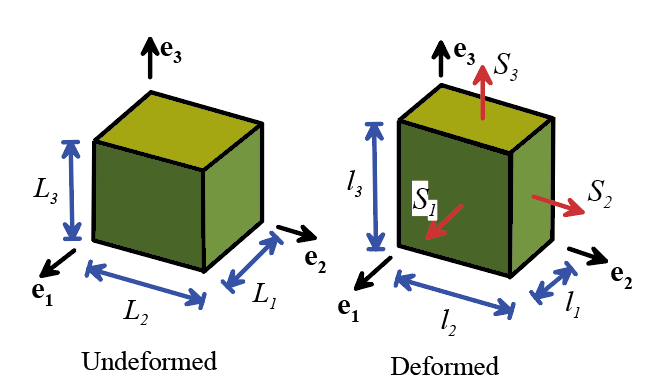
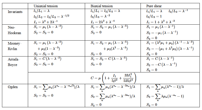
4. A more accurate description of material response to multiaxial loading can be obtained by fitting the material parameters to multiaxial tests.  To help in this exercise, the nominal stress (i.e. force/unit undeformed area) $–$v- extension predicted by several constitutive laws are listed in the table below (assuming perfectly incompressible behavior, as suggested in item 1.). Specimen dimensions are illustrated in the figure.

 

 

 

 

 

 

3.5.7 Representative values of material properties for rubbers

 

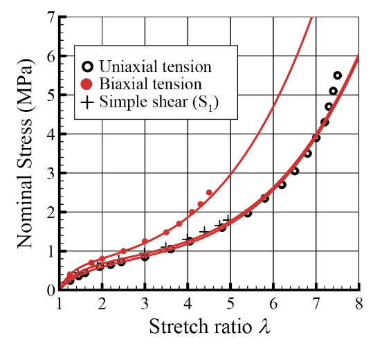The properties of rubber are strongly sensitive to its molecular structure, and for accurate predictions you will need to obtain experimental data for the particular material you plan to use.    As a rough guide, the experimental data of Treloar (1944) for the behavior of vulcanized rubber under uniaxial tension, biaxial tension, and pure shear is shown in the figure. The solid lines in the figure show the predictions of the Ogden model (which gives the best fit to the data).

 

Material parameters fit to this data for several constitutive laws are listed in the table below.