Chapter 4
Solutions to Simple Boundary and Initial Value Problems
for Elastic Solids

 

 

 

In this chapter, we derive exact solutions to several problems involving elastic solids.  The examples have been selected partly because they can easily be solved, partly because they illustrate clearly the role of the various governing equations and boundary conditions in controlling the solution, and partly because the solutions themselves are of some practical interest.

 

 

 

4.1 Axially and spherically symmetric solutions to quasi-static linear elastic problems

 

If an isotropic, linear elastic solid with spherical or cylindrical geometry is loaded so that it remains spherical or cylindrical after deformation, its shape and the internal stresses can usually be calculated by solving a straightforward ordinary differential equation for the displacement field.   This section derives the simplified equations for solids with the relevant geometry, and solves a few representative problems as examples.

 

 

 

4.1.1 Summary of governing equations of linear elasticity in Cartesian components

 

It is helpful to review briefly the equations we must solve in order to calculate deformation in an elastic material subjected to loading. 

 

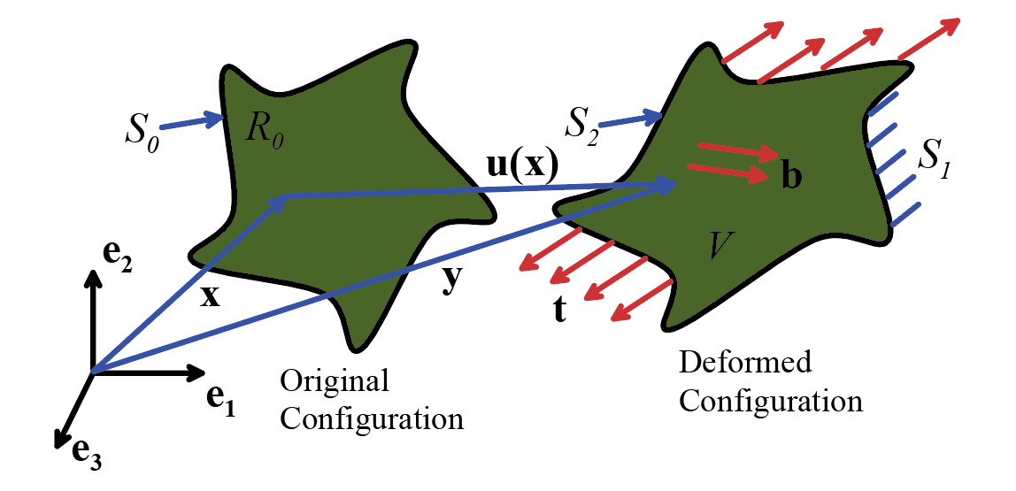A representative problem is sketched in the figure. We are given the following information

 

1. The geometry of the solid

 

2. A constitutive law for the material (i.e. the linear elastic-stress-strain equations)

 

3. Body force density $b_i$ (per unit mass) (if any)

 

4. Temperature distribution $\Delta T$ (if any)

 

5. Prescribed boundary tractions $t_i$ and/or boundary displacements $u_i$

 

 

In addition, to simplify the problem, we make the following assumptions

 

1. All displacements are small.  This means that we can use the infinitesimal strain tensor to characterize deformation; we do not need to distinguish between stress measures, and we do not need to distinguish between deformed and undeformed configurations of the solid when writing equilibrium equations and boundary conditions.

 

2. The material is an isotropic, linear elastic solid, with Young’s modulus E and Poisson’s ratio $\nu$, and mass density ${\rho }_0$

 

With these assumptions, we need to solve for the displacement field $u_i$, the strain field ${\epsilon }_{ij}$ and the stress field ${\sigma }_{ij}$ satisfying the following equations:

 

· Displacement$—$strain relation ${\epsilon }_{ij}={\displaystyle \frac{1}{2}\left({\displaystyle \frac{\partial u_i}{\partial x_j}+{\displaystyle \frac{\partial u_j}{\partial x_i}}}\right)}$

 

· Stress$—$strain relation ${\sigma }_{ij}={\displaystyle \frac{E}{1+\nu }\left\{{\epsilon }_{ij}+{\displaystyle \frac{\nu }{1-2\nu }{\epsilon }_{kk}{\delta }_{ij}}\right\}-{\displaystyle \frac{E\alpha \Delta T}{1-2\nu }{\delta }_{ij}}}$

 

 

· Equilibrium Equation $\partial {\sigma }_{ij}/\partial x_i+{\rho }_0{b}_j=0$ (static problems only $–$ you need the acceleration terms for dynamic problems)

 

· Traction boundary conditions ${\sigma }_{ij}{n}_i=t_j$ on parts of the boundary where tractions are known.

 

· Displacement boundary conditions $u_i=d_i$ on parts of the boundary where displacements are known.

 

 

 

4.1.2 Simplified equations for spherically symmetric linear elasticity problems

 

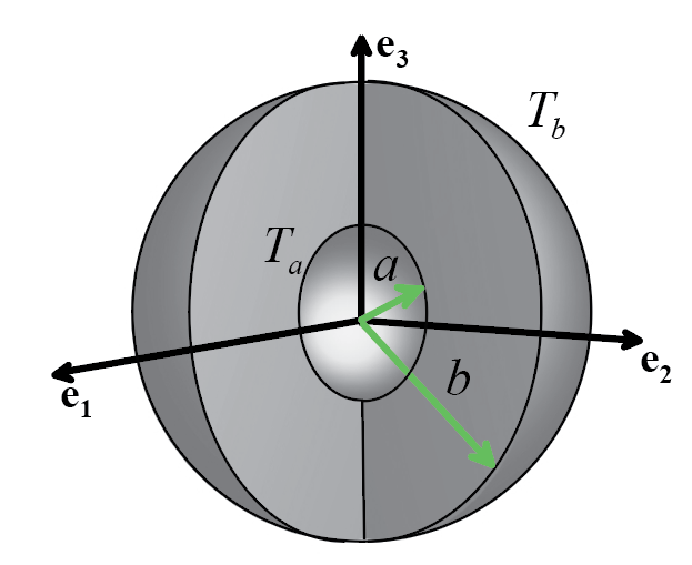
A representative spherically symmetric problem is illustrated in the figure.  We consider a hollow, spherical solid, which is subjected to spherically symmetric loading (i.e. internal body forces, as well as tractions or displacements applied to the surface, are independent of $\theta$ and $\varphi$, and act in the radial direction only).  If the temperature of the sphere is non-uniform, it must also be spherically symmetric (a function of R only).

 

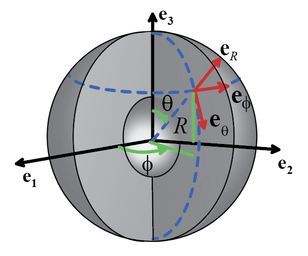
The solution is most conveniently expressed using a spherical-polar coordinate system, illustrated in the figure.  The general procedure for solving problems using spherical and cylindrical coordinates is complicated, and is discussed in detail in Appendix D.  In this section, we simply summarize the special form of these equations for spherically symmetric problems.

 

As usual, a point in the solid is identified by its spherical-polar co-ordinates $(R,\theta ,\varphi )$. All vectors and tensors are expressed as components in the basis $\left\{e_R,e_{\theta },e_{\varphi }\right\}$ shown in the figure.  For a spherically symmetric problem

 

· Position Vector       $x=R{e}_R$

 

· Displacement vector $u=u(R)e_R$

 

· Body force vector $b={\rho }_{0}b(R)e_R$

 

Here, $u\left(R\right)$ and $b\left(R\right)$ are scalar functions. The stress and strain tensors (written as components in $\{e_R,e_{\theta },e_{\varphi }\}$ ) have the form

$\sigma \equiv \left[\begin{array}{ccc}{\sigma }_{RR}& 0& 0\\ 0& {\sigma }_{\theta \theta }& 0\\ 0& 0& {\sigma }_{\varphi \varphi }\end{array}\right]\epsilon \equiv \left[\begin{array}{ccc}{\epsilon }_{RR}& 0& 0\\ 0& {\epsilon }_{\theta \theta }& 0\\ 0& 0& {\epsilon }_{\varphi \varphi }\end{array}\right]$

and furthermore must satisfy ${\sigma }_{\theta \theta }={\sigma }_{\varphi \varphi }$ ${\epsilon }_{\theta \theta }={\epsilon }_{\varphi \varphi }$. The tensor components have exactly the same physical interpretation as they did when we used a fixed $\{e_1,e_2,e_3\}$ basis, except that the subscripts (1,2,3) have been replaced by $(R,\theta ,\varphi )$.

 

For spherical symmetry, the governing equations of linear elasticity reduce to

 

· Strain Displacement Relations ${\epsilon }_{RR}={\displaystyle \frac{du}{dR}{\epsilon }_{\varphi \varphi }={\epsilon }_{\theta \theta }={\displaystyle \frac{u}{R}}}$

 

· Stress$—$Strain relations

$\begin{array}{l}{\sigma }_{RR}={\displaystyle \frac{E}{\left(1+\nu \right)\left(1-2\nu \right)}\left\{(1-\nu ){\epsilon }_{RR}+\nu {\epsilon }_{\theta \theta }+\nu {\epsilon }_{\varphi \varphi }\right\}-{\displaystyle \frac{E\alpha \Delta T}{1-2\nu }}}\\ {\sigma }_{\theta \theta }={\sigma }_{\varphi \varphi }={\displaystyle \frac{E}{\left(1+\nu \right)\left(1-2\nu \right)}\left\{{\epsilon }_{\theta \theta }+\nu {\epsilon }_{RR}\right\}-{\displaystyle \frac{E\alpha \Delta T}{1-2\nu }}}\end{array}$

 

·    Equilibrium Equations

${\displaystyle \frac{d{\sigma }_{RR}}{dR}+{\displaystyle \frac{1}{R}\left(2{\sigma }_{RR}-{\sigma }_{\theta \theta }-{\sigma }_{\varphi \varphi }\right)+{\rho }_0{b}_R=0}}$

 

·    Boundary Conditions

 

Prescribed Displacements $u_R(a)=g_a{u}_R(b)=g_b$

Prescribed Tractions ${\sigma }_{RR}(a)=t_a{\sigma }_{RR}(b)=t_b$

 

 

These results can either be derived as a special case of the general 3D equations of linear elasticity in spherical coordinates (see Appendix D), or alternatively can be obtained directly from the formulas in Cartesian components.  Here, we briefly outline the the latter.

 

1. Note that we can find the components of $\left\{e_R,e_{\theta },e_{\varphi }\right\}$ in the $\left\{e_1,e_2,e_3\right\}$ basis as follows. First, note that $e_R$ is radial, and can be written in terms of the position vector as $x/\left|x\right|$.  Next, note $e_{\varphi }=e_3\times e_R/\left|e_3\times e_R\right|$ and $e_{\theta }=e_{\varphi }\times e_R/\left|e_{\varphi }\times e_R\right|$.  Using index notation, the components of the basis vectors $\left\{e_R,e_{\theta },e_{\varphi }\right\}$ in $\left\{e_1,e_2,e_3\right\}$ are therefore

$\left\{{\displaystyle \frac{x_i}{R},{\displaystyle \frac{x_3{x}_i-R^2{\delta }_{i3}}{R^2-x_3^2},{\displaystyle \frac{{\in }_{i3j}R{x}_j}{R^2-x_3^2}}}}\right\}$

where $R=\left|x\right|=\sqrt{x_k{x}_k}$, ${\delta }_{ij}$ is the Kronecker delta and ${\in }_{ijk}$ is the permutation symbol.

 

2. The components of the (radial) displacement vector in the $\left\{e_1,e_2,e_3\right\}$ basis are $u_i=u(R)x_i/R$.

 

3. To proceed with the algebra, it is helpful to remember that $\partial x_i/\partial x_j={\delta }_{ij}$,  $\partial R/\partial x_j=x_j/R$ and $\partial R^{-1}/\partial x_j=-x_j/R^3$

 

 

4. The components of the strain tensor in the $\left\{e_1,e_2,e_3\right\}$ basis therefore follow as

${\epsilon }_{ij}={\displaystyle \frac{1}{2}\left({\displaystyle \frac{\partial u_i}{\partial x_j}+{\displaystyle \frac{\partial u_j}{\partial x_i}}}\right)={\displaystyle \frac{du}{dR}{\displaystyle \frac{x_i{x}_j}{R^2}+u(R)\left({\displaystyle \frac{{\delta }_{ij}}{R}-{\displaystyle \frac{x_i{x}_j}{R^3}}}\right)}}}$

 

5. The strain components ${\epsilon }_{RR},{\epsilon }_{\theta \theta },{\epsilon }_{\varphi \varphi }$ can then be found as ${\epsilon }_{RR}=e_R\cdot \epsilon e_R$, ${\epsilon }_{\theta \theta }=e_{\theta }\cdot \epsilon e_{\theta }$ and ${\epsilon }_{\varphi \varphi }=e_{\varphi }\cdot \epsilon e_{\varphi }$.  Substituting for the basis vectors and simplifying gives the strain-displacement relations.  For example

${\epsilon }_{RR}={\epsilon }_{ij}{\displaystyle \frac{x_i{x}_j}{R^2}={\displaystyle \frac{du}{dR}{\displaystyle \frac{x_i{x}_i{x}_j{x}_j}{R^4}+u(R)\left({\displaystyle \frac{{\delta }_{ij}}{R}{\displaystyle \frac{x_i{x}_j}{R^2}-{\displaystyle \frac{x_i{x}_i{x}_j{x}_j}{R^5}}}}\right)={\displaystyle \frac{du}{dR}}}}}$

where we have noted $x_i{x}_i=R^2$. The remaining components are left as an exercise.

 

6. Finally, to derive the equilibrium equation, note that the stress tensor can be expressed as $\sigma ={\sigma }_{RR}{e}_R\otimes e_R+{\sigma }_{\theta \theta }{e}_{\theta }\otimes e_{\theta }+{\sigma }_{\varphi \varphi }{e}_{\varphi }\otimes e_{\varphi }$.  Substituting for the basis vectors from item (1) above gives

${\sigma }_{ij}={\sigma }_{RR}{\displaystyle \frac{x_i{x}_j}{R^2}+{\sigma }_{\theta \theta }{\displaystyle \frac{{\in }_{i3k}R{x}_k}{R^2-x_3^2}{\displaystyle \frac{{\in }_{j3n}R{x}_n}{R^2-x_3^2}+{\sigma }_{\varphi \varphi }\left({\displaystyle \frac{x_3{x}_i-R^2{\delta }_{i3}}{R^2-x_3^2}}\right)\left({\displaystyle \frac{x_3{x}_j-R^2{\delta }_{j3}}{R^2-x_3^2}}\right)}}}$

 

7. Substitute the preceding result into the equilibrium equation

${\displaystyle \frac{\partial {\sigma }_{ij}}{\partial x_i}+{\rho }_{0}b(R){\displaystyle \frac{x_j}{R}=0}}$

and work through a good deal of tedious algebra to see that

$\left({\displaystyle \frac{d{\sigma }_{RR}}{dR}+{\displaystyle \frac{1}{R}\left(2{\sigma }_{RR}-{\sigma }_{\theta \theta }-{\sigma }_{\varphi \varphi }\right)+{\rho }_{0}b(R)}}\right){\displaystyle \frac{x_j}{R}=0}$

 

 

 

4.1.3 General solution to the spherically symmetric linear elasticity problem

 

Our goal is to solve the equations given in Section 4.1.2 for the displacement, strain and stress in the sphere.  To do so,

 

1. Substitute the strain-displacement relations into the stress-strain law to show that

$\left[\begin{array}{c}{\sigma }_{RR}\\ {\sigma }_{\theta \theta }\end{array}\right]={\displaystyle \frac{E}{\left(1+\nu \right)\left(1-2\nu \right)}\left[\begin{array}{cc}1-\nu & 2\nu \\ \nu & 1\end{array}\right]\left[\begin{array}{c}{\displaystyle \frac{du}{dR}}\\ {\displaystyle \frac{u}{R}}\end{array}\right]-{\displaystyle \frac{E\alpha \Delta T}{1-2\nu }\left[\begin{array}{c}1\\ 1\end{array}\right]}}$

 

2. Substitute this expression for the stress into the equilibrium equation and rearrange the result to see that

${\displaystyle \frac{d^{2}u}{d{R}^2}+{\displaystyle \frac{2}{R}{\displaystyle \frac{du}{dR}-{\displaystyle \frac{2u}{R^2}={\displaystyle \frac{d}{dR}\left\{{\displaystyle \frac{1}{R^2}{\displaystyle \frac{d}{dR}\left(R^{2}u\right)}}\right\}={\displaystyle \frac{\alpha \left(1+\nu \right)}{\left(1-\nu \right)}{\displaystyle \frac{d\Delta T}{dR}-{\displaystyle \frac{\left(1+\nu \right)\left(1-2\nu \right)}{E\left(1-\nu \right)}{\rho }_{0}b(R)}}}}}}}}$

 

 

Given the temperature distribution and body force this equation can easily be integrated to calculate the displacement u.  Two arbitrary constants of integration will appear when you do the integral $–$ these must be determined from the boundary conditions at the inner and outer surface of the sphere.  Specifically, the constants must be selected so that either the displacement or the radial stress have prescribed values on the inner and outer surface of the sphere.

 

In the following sections, this procedure is used to derive solutions to various boundary value problems of practical interest.

 

 

 

4.1.4 Pressurized hollow sphere

 

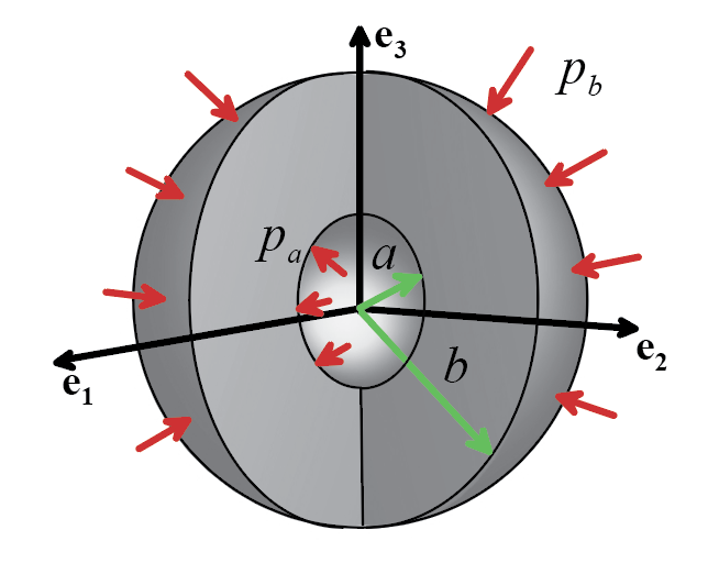A pressurized sphere is illustrated in the figure. Assume that

 

·    No body forces act on the sphere

 

·    The sphere has uniform temperature

 

 

·    The inner surface R=a is subjected to pressure $p_a$

 

·    The outer surface R=b is subjected to pressure $p_b$

 

 

 

The displacement, strain and stress fields in the sphere are

$u={\displaystyle \frac{1}{2E\left(b^3-a^3\right)R^2}\left\{2\left(p_a{a}^3-p_b{b}^3\right)\left(1-2\nu \right)R^3+\left(p_a-p_b\right)\left(1+\nu \right)b^3{a}^3\right\}{e}_R}$ ${\epsilon }_{RR}={\displaystyle \frac{1}{E\left(b^3-a^3\right)R^3}\left\{\left(p_a{a}^3-p_b{b}^3\right)\left(1-2\nu \right)R^3-\left(p_a-p_b\right)\left(1+\nu \right)b^3{a}^3\right\}}$

${\epsilon }_{\theta \theta }={\epsilon }_{\varphi \varphi }={\displaystyle \frac{1}{2E\left(b^3-a^3\right)R^3}\left\{2\left(p_a{a}^3-p_b{b}^3\right)\left(1-2\nu \right)R^3+\left(p_a-p_b\right)\left(1+\nu \right)b^3{a}^3\right\}}$

$\begin{array}{l}{\sigma }_{RR}={\displaystyle \frac{\left(p_a{a}^3-p_b{b}^3\right)}{\left(b^3-a^3\right)}-{\displaystyle \frac{\left(p_a-p_b\right)b^3{a}^3}{\left(b^3-a^3\right)R^3}}}\\ {\sigma }_{\theta \theta }={\sigma }_{\varphi \varphi }={\displaystyle \frac{\left(p_a{a}^3-p_b{b}^3\right)}{\left(b^3-a^3\right)}+{\displaystyle \frac{\left(p_a-p_b\right)b^3{a}^3}{2\left(b^3-a^3\right)R^3}}}\end{array}$    

 

Derivation:  The solution can be found by applying the procedure outlined in Sect 4.1.3.

 

1. Note that the governing equation for u (Sect 4.1.3) reduces to

${\displaystyle \frac{d}{dR}\left\{{\displaystyle \frac{1}{R^2}{\displaystyle \frac{d}{dR}\left(R^{2}u\right)}}\right\}=0}$

 

2. Integrating twice gives

$u=AR+{\displaystyle \frac{B}{R^2}}$

where A and B are constants of integration to be determined.

 

3. The radial stress follows by substituting into the stress-displacement formulas

$\begin{array}{l}{\sigma }_{RR}={\displaystyle \frac{E}{\left(1+\nu \right)\left(1-2\nu \right)}\left\{\left(1-\nu \right){\displaystyle \frac{du}{dR}+2\nu {\displaystyle \frac{u}{R}}}\right\}}\\ ={\displaystyle \frac{E}{\left(1+\nu \right)\left(1-2\nu \right)}\left\{\left(1+\nu \right)A-2\left(1-2\nu \right){\displaystyle \frac{B}{R^3}}\right\}}\end{array}$

 

4. To satisfy the boundary conditions, A and B must be chosen so that ${\sigma }_{RR}(R=a)=-p_a$ and ${\sigma }_{RR}(R=b)=-p_b$ (the stress is negative because the pressure is compressive).  This gives two equations for A and B that are easily solved to find

$A={\displaystyle \frac{\left(p_b{b}^3-p_a{a}^3\right)\left(1-2\nu \right)}{\left(a^3-b^3\right)E}B={\displaystyle \frac{\left(p_b-p_a\right)\left(1+\nu \right)b^3{a}^3}{2\left(a^3-b^3\right)E}}}$

 

5. Finally, expressions for displacement, strain and stress follow by substituting for A and B in the formula for u in (2), and using the formulas for strain and stress in terms of u in Section 4.1.2.

 

 

 

4.1.5 Gravitating sphere

 

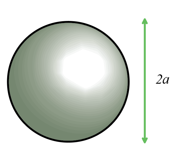A planet under its own gravitational attraction may be idealized (rather crudely) as a solid sphere with radius a, illustrated in the figure. The solid is subjected to the following loading

 

·    A body force $b=-(gR/a)e_R$ per unit mass, where g is the acceleration due to gravity at the surface of the sphere

 

·    A uniform temperature distribution

 

·    A traction free surface at R=a

 

 

The displacement, strain and stress in the sphere follow as

$u={\displaystyle \frac{\left(1-2\nu \right)}{10aE\left(1-\nu \right)}{\rho }_{0}gR\left\{\left(1+\nu \right)R^2-\left(3-\nu \right)a^2\right\}{e}_R}$

${\epsilon }_{RR}={\displaystyle \frac{\left(1-2\nu \right)}{10aE\left(1-\nu \right)}{\rho }_{0}g\left\{3\left(1+\nu \right)R^2-\left(3-\nu \right)a^2\right\}}$

${\epsilon }_{\theta \theta }={\epsilon }_{\varphi \varphi }={\displaystyle \frac{\left(1-2\nu \right)}{10aE\left(1-\nu \right)}{\rho }_{0}g\left\{\left(1+\nu \right)R^2-\left(3-\nu \right)a^2\right\}}$

$\begin{array}{l}{\sigma }_{RR}={\displaystyle \frac{{\rho }_{0}g(3-\nu )}{10a\left(1-\nu \right)}\left(R^2-a^2\right)}\\ {\sigma }_{\theta \theta }={\sigma }_{\varphi \varphi }={\displaystyle \frac{{\rho }_{0}g}{10a\left(1-\nu \right)}\left\{\left(3\nu +1\right)R^2-\left(3-\nu \right)a^2\right\}}\end{array}$           

 

Derivation:

 

1. Begin by writing the governing equation for u given in 4.1.3 as

${\displaystyle \frac{d}{dR}\left\{{\displaystyle \frac{1}{R^2}{\displaystyle \frac{d}{dR}\left(R^{2}u\right)}}\right\}={\displaystyle \frac{\left(1+\nu \right)\left(1-2\nu \right)}{E\left(1-\nu \right)}{\displaystyle \frac{{\rho }_{0}gR}{a}}}}$

 

2. Integrating

$u={\displaystyle \frac{\left(1+\nu \right)\left(1-2\nu \right)}{E\left(1-\nu \right)}{\displaystyle \frac{{\rho }_{0}g{R}^3}{10a}+AR+{\displaystyle \frac{B}{R^2}}}}$

where A and B are constants of integration that must be determined from boundary conditions.

 

3. The radial stress follows from the formulas in 4.1.3 as

$\begin{array}{l}{\sigma }_{RR}={\displaystyle \frac{E}{\left(1+\nu \right)\left(1-2\nu \right)}\left\{\left(1-\nu \right){\displaystyle \frac{du}{dR}+2\nu {\displaystyle \frac{u}{R}}}\right\}}\\ ={\displaystyle \frac{{\rho }_{0}g(3-\nu )R^2}{10a(1-\nu )}+{\displaystyle \frac{E}{\left(1+\nu \right)\left(1-2\nu \right)}\left\{\left(1+\nu \right)A-2\left(1-2\nu \right){\displaystyle \frac{B}{R^3}}\right\}}}\end{array}$

 

4. Finally, the constants A and B can be determined as follows: (i) The stress must be finite at $R\to 0$, which is only possible if $B=0$.  (ii) The surface of the sphere is traction free, which requires ${\sigma }_{RR}=0$ at R=a.  Substituting the latter condition into the formula for stress in (3) and solving for A gives

$A=-{\displaystyle \frac{\left(1-2\nu \right)\left(3-\nu \right){\rho }_{0}ga}{10E(1-\nu )}}$

 

5. The final formulas for stress and strain follow by substituting the result of (4) back into (2), and using the formulas in Section 4.1.2.

 

 

 

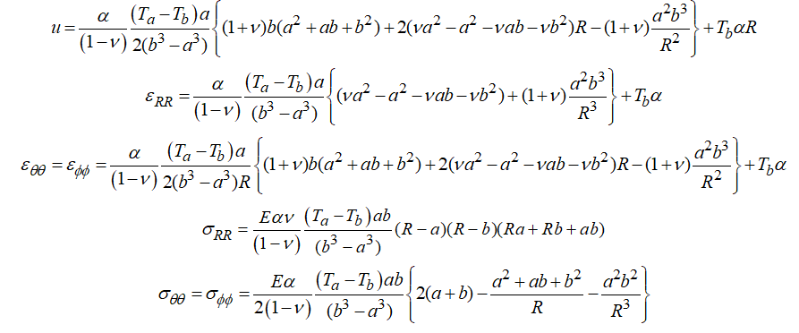
4.1.6 Sphere with steady state heat flow

 

The deformation and stress in a sphere that is heated on the inside (or outside), and has reached its steady state temperature distribution can be calculated as follows.  A hollow sphere is shown in the figure. Assume that

 

· No body force acts on the sphere

 

· The temperature distribution in the sphere is

$T={\displaystyle \frac{T_{b}b-T_{a}a}{b-a}+{\displaystyle \frac{\left(T_a-T_b\right)ab}{(b-a)R}}}$

where $T_a$ and $T_b$ are the temperatures at the inner and outer surfaces.  The total rate of heat loss from the sphere is $\dot{Q}=4\pi k(T_a-T_b)ab/(b-a)$, where k is the thermal conductivity.

 

· The surfaces at R=a  and R=b are traction free.

 

 

The displacement, strain and stress fields in the sphere follow as

 

 

Derivation:

 

1. The differential equation for u given in 4.1.3 reduces to

${\displaystyle \frac{d}{dR}\left\{{\displaystyle \frac{1}{R^2}{\displaystyle \frac{d}{dR}\left(R^{2}u\right)}}\right\}=-{\displaystyle \frac{\alpha \left(1+\nu \right)}{\left(1-\nu \right)}{\displaystyle \frac{\left(T_a-T_b\right)ab}{(b-a)R^2}}}}$

 

2. Integrating

$u={\displaystyle \frac{\alpha \left(1+\nu \right)}{2\left(1-\nu \right)}{\displaystyle \frac{\left(T_a-T_b\right)ab}{(b-a)}+AR+{\displaystyle \frac{B}{R^2}}}}$

where A and B are constants of integration.

 

3. The radial stress follows from the formulas in 4.1.3 as

$\begin{array}{l}{\sigma }_{RR}={\displaystyle \frac{E}{\left(1+\nu \right)\left(1-2\nu \right)}\left\{\left(1-\nu \right){\displaystyle \frac{du}{dR}+2\nu {\displaystyle \frac{u}{R}}}\right\}-{\displaystyle \frac{E\alpha \Delta T}{1-2\nu }}}\\ ={\displaystyle \frac{E\nu \alpha }{\left(1-2\nu \right)\left(1-\nu \right)}{\displaystyle \frac{\left(T_a-T_b\right)ab}{(b-a)R}+{\displaystyle \frac{E}{\left(1+\nu \right)\left(1-2\nu \right)}\left\{\left(1+\nu \right)A-2\left(1-2\nu \right){\displaystyle \frac{B}{R^3}}\right\}}}}\\ -{\displaystyle \frac{E\alpha }{1-2\nu }\left\{{\displaystyle \frac{T_{b}b-T_{a}a}{b-a}+{\displaystyle \frac{\left(T_a-T_b\right)ab}{(b-a)R}}}\right\}}\end{array}$

 

4. The boundary conditions require that ${\sigma }_{rr}=0$ at r=a and r=b.  Substituting these conditions into the result of step (3) gives two equations for A and B which can be solved to see that

$\begin{array}{l}A={\displaystyle \frac{(1-\nu )(T_b{b}^3-T_a{a}^3)+(T_a-T_b)\nu ab(a+b)}{\left(1-\nu \right)\left(a^3-b^3\right)}}\\ B={\displaystyle \frac{\alpha \left(T_a-T_b\right)\left(1+\nu \right)}{2\left(1-\nu \right)}{\displaystyle \frac{a^3{b}^3}{\left(b^3-a^3\right)}}}\end{array}$

 

 

 

4.1.7 Simplified equations for axially symmetric linear elasticity problems

 

Two examples of axially symmetric problems are illustrated below.  In both cases the solid is a circular cylinder, which is subjected to axially symmetric loading (i.e. internal body forces, as well as tractions or displacements applied to the surface, are independent of $\theta$ and $z$, and act in the radial direction only).  If the temperature of the sphere is non-uniform, it must also be axially symmetric (a function of r only).  Finally, the solid can spin with steady angular velocity about the $e_3$ axis.

 

 

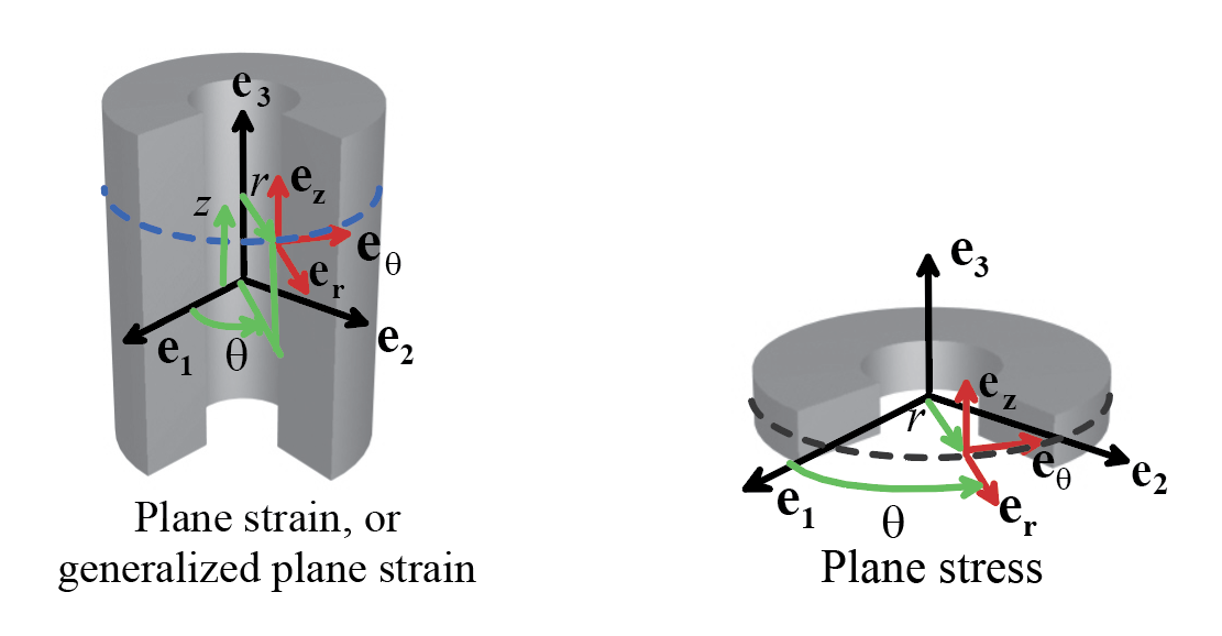
The two solids have different shapes.  In the first case, the length of the cylinder is substantially greater than any cross-sectional dimension.  In the second case, the length of the cylinder is much less than its outer radius. 

 

The state of stress and strain in the solid depends on the loads applied to the ends of the cylinder. Specifically

 

· If the cylinder is completely prevented from stretching in the $e_3$ direction a state of plane strain exists in the solid.  This is an exact solution to the 3D equations of elasticity, is valid for a cylinder with any length, and is accurate everywhere in the cylinder.

 

· If the top and bottom surface of the short plate-like cylinder are free of traction, a state of plane stress exists in the solid.  This is an approximate solution to the 3D equations of elasticity, and is accurate only if the cylinder’s length is much less than its diameter.   

 

· If the top and bottom  ends of the long cylinder are subjected to a prescribed force (or the ends are free of force) a state of generalized plane strain exists in the cylinder.  This is an approximate solution, which is accurate only away from the ends of a long cylinder.  As a rule of thumb, the solution is applicable approximately three cylinder radii away from the ends.

 

 

The solution is most conveniently expressed using a cylindrical-polar coordinate system, illustrated in Figure 4.6.  A point in the solid is identified by its spherical-polar co-ordinates $(r,\theta ,z)$. All vectors and tensors are expressed as components in the basis $\left\{e_r,e_{\theta },e_z\right\}$ shown in the figure.  For an axially symmetric problem

 

· Position Vector       $x=r{e}_r+z{e}_z$

 

· Displacement vector $u=u(r)e_r+{\epsilon }_{zz}z{e}_z$

 

· Body force vector $b={\rho }_{0}b(r)e_r$

 

· Acceleration vector $a=-{\omega }^{2}r$

 

 

Here, $u\left(r\right)$ and $b\left(r\right)$ are scalar functions.

 

The stress and strain tensors (written as components in $\{e_r,e_{\theta },e_z\}$ ) have the form

$\sigma \equiv \left[\begin{array}{ccc}{\sigma }_{rr}& 0& 0\\ 0& {\sigma }_{\theta \theta }& 0\\ 0& 0& {\sigma }_{zz}\end{array}\right]\epsilon \equiv \left[\begin{array}{ccc}{\epsilon }_{rr}& 0& 0\\ 0& {\epsilon }_{\theta \theta }& 0\\ 0& 0& {\epsilon }_{zz}\end{array}\right]$

 

For axial symmetry, the governing equations of linear elasticity reduce to

 

· Strain Displacement Relations ${\epsilon }_{rr}={\displaystyle \frac{du}{dr}{\epsilon }_{\theta \theta }={\displaystyle \frac{u}{r}}}$

 

· Stress$—$Strain relations (plane strain and generalized plane strain)

$\left[\begin{array}{c}{\sigma }_{rr}\\ {\sigma }_{\theta \theta }\\ {\sigma }_{zz}\end{array}\right]={\displaystyle \frac{E}{(1+\nu )(1-2\nu )}\left[\begin{array}{ccc}1-\nu & \nu & \nu \\ \nu & 1-\nu & \nu \\ \nu & \nu & 1-\nu \end{array}\right]\left[\begin{array}{c}{\epsilon }_{rr}\\ {\epsilon }_{\theta \theta }\\ {\epsilon }_{zz}\end{array}\right]-{\displaystyle \frac{E\alpha \Delta T}{1-2\nu }\left[\begin{array}{c}1\\ 1\\ 1\end{array}\right]}}$

    where ${\epsilon }_{zz}=0$ for plane strain, and constant for generalized plane strain.

 

· Stress$—$Strain relations (plane stress)

$\left[\begin{array}{c}{\sigma }_{rr}\\ {\sigma }_{\theta \theta }\end{array}\right]={\displaystyle \frac{E}{1-{\nu }^2}\left[\begin{array}{cc}1& \nu \\ \nu & 1\end{array}\right]\left[\begin{array}{c}{\epsilon }_{rr}\\ {\epsilon }_{\theta \theta }\end{array}\right]-{\displaystyle \frac{E\alpha \Delta T}{1-\nu }\left[\begin{array}{c}1\\ 1\end{array}\right]}}$

${\sigma }_{zz}=0{\epsilon }_{zz}=-{\displaystyle \frac{\nu }{E}\left({\sigma }_{rr}+{\sigma }_{\theta \theta }\right)+\alpha \Delta T}$

 

· Equation of motion

${\displaystyle \frac{d{\sigma }_{rr}}{dr}+{\displaystyle \frac{1}{r}\left({\sigma }_{rr}-{\sigma }_{\theta \theta }\right)+{\rho }_0{b}_r=-{\rho }_0{\omega }^{2}r}}$

 

· Boundary Conditions

 

Prescribed Displacements $u_r(a)=g_a{u}_r(b)=g_b$

Prescribed Tractions ${\sigma }_{rr}(a)=t_a{\sigma }_{rr}(b)=t_b$

Plane strain solution ${\epsilon }_{zz}=0$

Generalized plane strain solution, with axial force $F_z$ applied to cylinder:

${\displaystyle \underset{a}{\overset{b}{\int }}2\pi r{\sigma }_{zz}}dr=F_z$

 

These results can either be derived as a special case of the general 3D equations of linear elasticity in spherical coordinates, or alternatively can be obtained directly from the formulas in Cartesian components.  Here, we briefly outline the the latter.

 

1. Note that we can find the components of $\left\{e_r,e_{\theta },e_z\right\}$ in the $\left\{e_1,e_2,e_3\right\}$ basis as follows. First, note that $e_r$ is radial $–$ a radial unit vector can be written in terms of the position vector as $x/\left|x\right|$.  Next, note $e_{\theta }=e_3\times e_r$ and $e_z=e_3$.  Using index notation, the components of the basis vectors $\left\{e_r,e_{\theta },e_z\right\}$ in $\left\{e_1,e_2,e_3\right\}$ are therefore

$\left\{{\displaystyle \frac{x_{\alpha }}{r},{\in }_{i3\alpha }{\displaystyle \frac{x_{\alpha }}{r},{\delta }_{i3}}}\right\}$

where $r=\sqrt{x_{\alpha }{x}_{\alpha }}=\sqrt{x_1^2+x_2^2}$, and we use the convention that Greek subscripts range from 1 to 2

 

2. The components of the (radial) displacement vector in the $\left\{e_1,e_2,e_3\right\}$ basis are $u_{\alpha }=u(r)x_{\alpha }/r$.

 

3. To proceed with the algebra, it is helpful to remember that $\partial x_{\alpha }/\partial x_{\alpha }={\delta }_{\alpha \beta }$,  $\partial r/\partial x_{\alpha }=x_{\alpha }/r$ and $\partial r^{-1}/\partial x_{\alpha }=-x_{\alpha }/r^3$

 

4. The components of the strain tensor in the $\left\{e_1,e_2,e_3\right\}$ basis therefore follow as

${\epsilon }_{\alpha \beta }={\displaystyle \frac{1}{2}\left({\displaystyle \frac{\partial u_{\alpha }}{\partial x_{\beta }}+{\displaystyle \frac{\partial u_{\beta }}{\partial x_{\alpha }}}}\right)={\displaystyle \frac{du}{dr}{\displaystyle \frac{x_{\alpha }{x}_{\beta }}{r^2}+u(r)\left({\displaystyle \frac{{\delta }_{\alpha \beta }}{r}-{\displaystyle \frac{x_{\alpha }{x}_{\beta }}{r^3}}}\right){\epsilon }_{zz}={\epsilon }_{33}}}}$

 

5. The strain components ${\epsilon }_{rr},{\epsilon }_{\theta \theta },{\epsilon }_{zz}$ can then be found as ${\epsilon }_{rr}=e_r\cdot \epsilon e_r$, ${\epsilon }_{\theta \theta }=e_{\theta }\cdot \epsilon e_{\theta }$ and ${\epsilon }_{zz}=e_z\cdot \epsilon e_z$.  Substituting for the basis vectors and simplifying gives the strain-displacement relations.  For example

${\epsilon }_{rr}={\epsilon }_{\alpha \beta }{\displaystyle \frac{x_{\alpha }{x}_{\beta }}{r^2}={\displaystyle \frac{du}{dr}{\displaystyle \frac{x_{\alpha }{x}_{\alpha }{x}_{\beta }{x}_{\beta }}{r^4}+u(r)\left({\displaystyle \frac{{\delta }_{\alpha \beta }}{r}{\displaystyle \frac{x_{\alpha }{x}_{\beta }}{r^2}-{\displaystyle \frac{x_{\alpha }{x}_{\alpha }{x}_{\beta }{x}_{\beta }}{r^5}}}}\right)={\displaystyle \frac{du}{dr}}}}}$

where we have noted $x_{\alpha }{x}_{\alpha }=r^2$. The remaining components are left as an exercise.

 

6. Finally, to derive the equilibrium equation, note that the stress tensor can be expressed as $\sigma ={\sigma }_{rr}{e}_r\otimes e_r+{\sigma }_{\theta \theta }{e}_{\theta }\otimes e_{\theta }+{\sigma }_{zz}{e}_z\otimes e_z$.  Substituting for the basis vectors from item(1) above gives

${\sigma }_{\alpha \beta }={\sigma }_{rr}{\displaystyle \frac{x_{\alpha }{x}_{\beta }}{r^2}+{\sigma }_{\theta \theta }{\in }_{i3\gamma }{\displaystyle \frac{x_{\gamma }}{r}{\in }_{\beta 3\kappa }{\displaystyle \frac{x_{\kappa }}{r}{\sigma }_{zz}={\sigma }_{33}}}}$

 

7. Substitute the preceding result into the equilibrium equation

${\displaystyle \frac{\partial {\sigma }_{ij}}{\partial x_i}+{\rho }_{0}b(r){\displaystyle \frac{x_j}{r}=0}}$

and crank through a good deal of tedious algebra to see that

$\left({\displaystyle \frac{d{\sigma }_{rr}}{dr}+{\displaystyle \frac{1}{r}\left({\sigma }_{rr}-{\sigma }_{\theta \theta }\right)+{\rho }_{0}b(r)}}\right){\displaystyle \frac{x_{\alpha }}{r}=0}$

 

 

 

4.1.8 General solution to the axisymmetric boundary value problem

 

Our goal is to solve the equations given in Section 4.1.2 for the displacement, strain and stress in the sphere.  To do so,

 

1.  Substitute the strain-displacement relations into the stress-strain law to show that, for generalized plane strain

$\left[\begin{array}{c}{\sigma }_{rr}\\ {\sigma }_{\theta \theta }\\ {\sigma }_{zz}\end{array}\right]={\displaystyle \frac{E}{(1+\nu )(1-2\nu )}\left[\begin{array}{ccc}1-\nu & \nu & \nu \\ \nu & 1-\nu & \nu \\ \nu & \nu & 1-\nu \end{array}\right]\left[\begin{array}{c}{\displaystyle \frac{du}{dr}}\\ {\displaystyle \frac{u}{r}}\\ {\epsilon }_{zz}\end{array}\right]-{\displaystyle \frac{E\alpha \Delta T}{1-2\nu }\left[\begin{array}{c}1\\ 1\\ 1\end{array}\right]}}$

where ${\epsilon }_{zz}$ is constant.  The equivalent expression for plane stress is

$\left[\begin{array}{c}{\sigma }_{rr}\\ {\sigma }_{\theta \theta }\end{array}\right]={\displaystyle \frac{E}{1-{\nu }^2}\left[\begin{array}{cc}1& \nu \\ \nu & 1\end{array}\right]\left[\begin{array}{c}{\displaystyle \frac{du}{dr}}\\ {\displaystyle \frac{u}{r}}\end{array}\right]-{\displaystyle \frac{E\alpha \Delta T}{1-\nu }\left[\begin{array}{c}1\\ 1\end{array}\right]}}$

 

2.  Substitute these expressions for the stress into the equilibrium equation and rearrange the result to see that, for generalized plane strain

$\begin{array}{l}{\displaystyle \frac{{\partial }^{2}u}{\partial r^2}+{\displaystyle \frac{1}{r}{\displaystyle \frac{\partial u}{\partial r}-{\displaystyle \frac{u}{r^2}={\displaystyle \frac{\partial }{\partial r}\left\{{\displaystyle \frac{1}{r}{\displaystyle \frac{\partial }{\partial r}\left(ru\right)}}\right\}}}}}}\\ ={\displaystyle \frac{\alpha \left(1+\nu \right)}{\left(1-\nu \right)}{\displaystyle \frac{\partial \Delta T}{\partial r}-{\displaystyle \frac{\left(1+\nu \right)\left(1-2\nu \right)}{E(1-\nu )}{\rho }_0(b+{\omega }^{2}r)}}}\end{array}$

while for plane stress

$\begin{array}{l}{\displaystyle \frac{{\partial }^{2}u}{\partial r^2}+{\displaystyle \frac{1}{r}{\displaystyle \frac{\partial u}{\partial r}-{\displaystyle \frac{u}{r^2}={\displaystyle \frac{\partial }{\partial r}\left\{{\displaystyle \frac{1}{r}{\displaystyle \frac{\partial }{\partial r}\left(ru\right)}}\right\}}}}}}\\ =\alpha \left(1+\nu \right){\displaystyle \frac{\partial \Delta T}{\partial r}-{\displaystyle \frac{\left(1-{\nu }^2\right)}{E}{\rho }_0(b+{\omega }^{2}r)}}\end{array}$

 

Given the temperature distribution and body force these equations can be integrated to calculate the displacement u.  Two arbitrary constants of integration will appear when you do the integral $–$ these must be determined from the boundary conditions at the inner and outer surface of the cylinder.  Specifically, the constants must be selected so that either the displacement or the radial stress have prescribed values on the inner and outer surface of the sphere.  Finally, for the generalized plane strain solution, the axial strain ${\epsilon }_{zz}$ must be determined, using the equation for the axial force acting on the ends of the cylinder.

 

In the following sections, this procedure is used to derive solutions to various boundary value problems of practical interest.

 

 

 

4.1.9 Long (generalized plane strain) cylinder subjected to internal and external pressure.

 

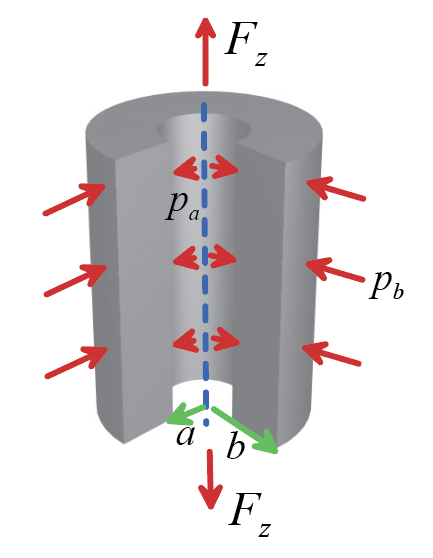We consider a long hollow cylinder with internal radius a and external radius b as shown in the figure.  Assume that

 

· No body forces act on the cylinder

 

· The cylinder has zero angular velocity

 

· The sphere has uniform temperature

 

· The inner surface r=a is subjected to pressure $p_a$

 

· The outer surface r=b is subjected to pressure $p_b$

 

· For the plane strain solution, the cylinder does not stretch parallel to its axis.  For the generalized plane strain solution, the ends of the cylinder are subjected to an axial force $F_z$ as shown.  In particular, for a closed ended cylinder the axial force exerted by the pressure inside the cylinder acting on the closed ends is $F_z=\pi \left(p_a{a}^2-p_b{b}^2\right)$

 

The displacement, strain and stress fields in the cylinder are

$u={\displaystyle \frac{\left(1+\nu \right)a^2{b}^2}{E\left(b^2-a^2\right)}\left\{{\displaystyle \frac{\left(p_a-p_b\right)}{r}+\left(1-2\nu \right){\displaystyle \frac{\left(p_a{a}^2-p_b{b}^2\right)}{a^2{b}^2}r}}\right\}{e}_r-\nu {\epsilon }_{zz}r{e}_r+{\epsilon }_{zz}z{e}_z}$

$\begin{array}{l}{\epsilon }_{rr}={\displaystyle \frac{\left(1+\nu \right)a^2{b}^2}{E\left(b^2-a^2\right)}\left\{-{\displaystyle \frac{\left(p_a-p_b\right)}{r^2}+\left(1-2\nu \right){\displaystyle \frac{\left(p_a{a}^2-p_b{b}^2\right)}{a^2{b}^2}}}\right\}-\nu {\epsilon }_{zz}}\\ {\epsilon }_{\theta \theta }={\displaystyle \frac{\left(1+\nu \right)a^2{b}^2}{E\left(b^2-a^2\right)}\left\{{\displaystyle \frac{\left(p_a-p_b\right)}{r^2}+\left(1-2\nu \right){\displaystyle \frac{\left(p_a{a}^2-p_b{b}^2\right)}{a^2{b}^2}}}\right\}-\nu {\epsilon }_{zz}}\end{array}$

$\begin{array}{l}{\sigma }_{rr}=\left\{{\displaystyle \frac{\left(p_a{a}^2-p_b{b}^2\right)}{b^2-a^2}-{\displaystyle \frac{a^2{b}^2}{\left(b^2-a^2\right)r^2}\left(p_a-p_b\right)}}\right\}\\ {\sigma }_{\theta \theta }=\left\{{\displaystyle \frac{\left(p_a{a}^2-p_b{b}^2\right)}{b^2-a^2}+{\displaystyle \frac{a^2{b}^2}{\left(b^2-a^2\right)r^2}\left(p_a-p_b\right)}}\right\}\\ {\sigma }_{zz}=2\nu {\displaystyle \frac{\left(p_a{a}^2-p_b{b}^2\right)}{b^2-a^2}+E{\epsilon }_{zz}}\end{array}$

where ${\epsilon }_{zz}=0$ for plane strain, while

${\epsilon }_{zz}={\displaystyle \frac{F_z}{\pi E(b^2-a^2)}-{\displaystyle \frac{2\nu }{E}{\displaystyle \frac{\left(p_a{a}^2-p_b{b}^2\right)}{(b^2-a^2)}}}}$

for generalized plane strain.

 

 

Derivation: These results can be derived as follows.  The governing equation reduces to

${\displaystyle \frac{{\partial }^{2}u}{\partial r^2}+{\displaystyle \frac{1}{r}{\displaystyle \frac{\partial u}{\partial r}-{\displaystyle \frac{u}{r^2}={\displaystyle \frac{\partial }{\partial r}\left\{{\displaystyle \frac{1}{r}{\displaystyle \frac{\partial }{\partial r}\left(ru\right)}}\right\}=0}}}}}$

The equation can be integrated to see that

$u=Ar+{\displaystyle \frac{B}{r}}$

The radial stress follows as

${\sigma }_{rr}={\displaystyle \frac{E}{\left(1+\nu \right)\left(1-2\nu \right)}\left\{(1-\nu ){\displaystyle \frac{\partial u}{\partial r}+\nu {\displaystyle \frac{u}{r}}}\right\}={\displaystyle \frac{E}{\left(1+\nu \right)\left(1-2\nu \right)}\left\{A-(1-2\nu ){\displaystyle \frac{B}{r^2}}\right\}}}$

The boundary conditions are ${\sigma }_{rr}(r=a)=-p_a{\sigma }_{rr}(r=b)=-p_b$ (the stresses are negative because the pressure is compressive).  This yields two equations for A and B that area easily solved to see that

$A={\displaystyle \frac{\left(1+\nu \right)\left(1-2\nu \right)}{E}{\displaystyle \frac{\left(p_a{a}^2-p_b{b}^2\right)}{b^2-a^2}B={\displaystyle \frac{\left(1+\nu \right)}{E}{\displaystyle \frac{a^2{b}^2}{b^2-a^2}\left(p_a-p_b\right)}}}}$

The remaining results follow by elementary algebraic manipulations.

 

 

 

4.1.10 Spinning circular plate

 

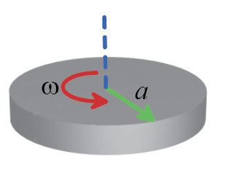We consider a thin solid plate with radius a that spins with angular speed $\omega$ about its axis, as shown in the figure.  Assume that

 

· No body forces act on the disk

 

· The disk has constant angular velocity

 

· The disk has uniform temperature

 

· The outer surface r=a and the top and bottom faces of the disk are free of traction.

 

· The disk is sufficiently thin to ensure a state of plane stress in the disk.

$u=(1-\nu ){\displaystyle \frac{{\rho }_0{\omega }^2}{8E}\left\{\left(3+\nu \right)a^{2}r-\left(1+\nu \right)r^3\right\}{e}_r+z{\epsilon }_{zz}{e}_z}$

$\begin{array}{l}{\epsilon }_{rr}=(1-\nu ){\displaystyle \frac{{\rho }_0{\omega }^2}{8E}\left\{\left(3+\nu \right)a^2-3\left(1+\nu \right)r^2\right\}}\\ {\epsilon }_{\theta \theta }=(1-\nu ){\displaystyle \frac{{\rho }_0{\omega }^2}{8E}\left\{\left(3+\nu \right)a^2-\left(1+\nu \right)r^2\right\}}\end{array}$          

${\epsilon }_{zz}=-\nu {\displaystyle \frac{{\rho }_0{\omega }^2}{4E}\left\{\left(3+\nu \right)a^2-2(1+\nu )r^2\right\}}$

$\begin{array}{l}{\sigma }_{rr}=\left(3+\nu \right){\displaystyle \frac{{\rho }_0{\omega }^2}{8}\left\{a^2-r^2\right\}}\\ {\sigma }_{\theta \theta }={\displaystyle \frac{{\rho }_0{\omega }^2}{8}\left\{(3+\nu )a^2-(3\nu +1)r^2\right\}}\end{array}$

 

Derivation: To derive these results, recall that the governing equation is

${\displaystyle \frac{{\partial }^{2}u}{\partial r^2}+{\displaystyle \frac{1}{r}{\displaystyle \frac{\partial u}{\partial r}-{\displaystyle \frac{u}{r^2}={\displaystyle \frac{\partial }{\partial r}\left\{{\displaystyle \frac{1}{r}{\displaystyle \frac{\partial }{\partial r}\left(ru\right)}}\right\}=-{\displaystyle \frac{\left(1-{\nu }^2\right)}{E}{\rho }_0{\omega }^{2}r}}}}}}$

The equation can be integrated to see that

$u=Ar+{\displaystyle \frac{B}{r}-{\displaystyle \frac{\left(1-{\nu }^2\right)}{8E}{\rho }_0{\omega }^2{r}^3}}$

The displacement must be bounded at r=0, which is only possible if B=0.   With this substitution, the radial stress follows as

${\sigma }_{rr}={\displaystyle \frac{E}{1-{\nu }^2}\left({\displaystyle \frac{du}{dr}+\nu {\displaystyle \frac{u}{r}}}\right)={\displaystyle \frac{E\left(1+\nu \right)}{1-{\nu }^2}\left\{A-{\displaystyle \frac{{\rho }_0{\omega }^2}{8E}\left(3+\nu \right)\left(1-\nu \right)r^2}\right\}}}$

The radial stress must be zero at r=a, which requires that

$A={\displaystyle \frac{{\rho }_0{\omega }^2}{8E}\left(3+\nu \right)(1-\nu )a^2}$

The remaining results follow by straightforward algebra.

 

 

 

4.1.11 Stresses induced by an interference fit between two cylinders

 

Interference fits are often used to secure a bushing or a bearing housing to a shaft.  In this problem we calculate the stress induced by such an interference fit.

 

 

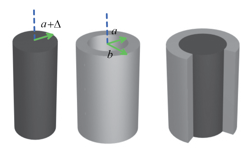
Consider a hollow cylindrical bushing, with outer radius b and inner radius a.  Suppose that a solid shaft with radius $a+\Delta$, with $\Delta /a<<1$ is inserted into the cylinder as shown above  (In practice, this is done by heating the cylinder or cooling the shaft until they fit, and then letting the system return to thermal equilibrium)

 

· No body forces act on the solids

 

· The angular velocity is zero

 

· The cylinders have uniform temperature

 

· The shaft slides freely inside the bushing

 

· The ends of the cylinder are free of force.

 

· Both the shaft and cylinder have the same Young’s modulus E and Poisson’s ratio $\nu$

 

· The cylinder and shaft are sufficiently long to ensure that a state of generalized plane strain can be developed in each solid.

 

 

The displacements, strains and stresses in the solid shaft  (r<a) are

$u=-{\displaystyle \frac{\left(1+\nu \right)\left(1-2\nu \right)\Delta (b^2-a^2)}{2a{b}^2}r{e}_r-2{\nu }^2{\displaystyle \frac{\Delta (b^2-a^2)}{2a{b}^2}r{e}_r+2\nu {\displaystyle \frac{\Delta (b^2-a^2)}{2a{b}^2}z{e}_z}}}$

${\epsilon }_{rr}={\epsilon }_{\theta \theta }=-{\displaystyle \frac{\left(1+\nu \right)\left(1-2\nu \right)\Delta (b^2-a^2)}{2a{b}^2}-2{\nu }^2{\displaystyle \frac{\Delta (b^2-a^2)}{2a{b}^2}}}$

${\sigma }_{rr}={\sigma }_{\theta \theta }=-{\displaystyle \frac{E\Delta (b^2-a^2)}{2a{b}^2}{\sigma }_{zz}=0}$

In the hollow cylinder, they are

$u={\displaystyle \frac{\left(1+\nu \right)a}{r}{\displaystyle \frac{\Delta }{2}\left\{1+\left(1-2\nu \right){\displaystyle \frac{r^2}{b^2}}\right\}{e}_r-{\nu }^2{\displaystyle \frac{\Delta a}{b^2}r{e}_r+2{\nu }^2{\displaystyle \frac{\Delta a}{b^2}z{e}_z}}}}$

$\begin{array}{l}{\epsilon }_{rr}={\displaystyle \frac{\left(1+\nu \right)a}{r^2}{\displaystyle \frac{\Delta }{2}\left\{-1+\left(1-2\nu \right){\displaystyle \frac{r^2}{b^2}}\right\}-{\nu }^2{\displaystyle \frac{\Delta a}{b^2}}}}\\ {\epsilon }_{\theta \theta }={\displaystyle \frac{\left(1+\nu \right)a}{r^2}{\displaystyle \frac{\Delta }{2}\left\{1+\left(1-2\nu \right){\displaystyle \frac{r^2}{b^2}}\right\}-{\nu }^2{\displaystyle \frac{\Delta a}{b^2}}}}\end{array}$

${\sigma }_{rr}={\displaystyle \frac{E\Delta a}{2b^2}\left\{1-{\displaystyle \frac{b^2}{r^2}}\right\}{\sigma }_{\theta \theta }={\displaystyle \frac{E\Delta a}{2b^2}\left\{1+{\displaystyle \frac{b^2}{r^2}}\right\}{\sigma }_{zz}=0}}$

 

 

Derivation: These results can be derived using the solution to a pressurized cylinder given in Section 4.1.9. After the shaft is inserted into the tube, a pressure p acts to compress the shaft, and the same pressure pushes outwards to expand the cylinder.  Suppose that this pressure induces a radial displacement $u^s(r)$ in the solid cylinder, and a radial displacement $u^c(r)$ in the hollow tube.  To accommodate the interference, the displacements must satisfy

$u^c(r=a)-u^s(r=a)=\Delta$

Evaluating the relevant displacements using the formulas in 4.1.9 gives

$\begin{array}{l}{u}^s(r=a)=-{\displaystyle \frac{\left(1-2\nu \right)\left(1+\nu \right)}{E}pa-{\displaystyle \frac{2{\nu }^2}{E}pa}}\\ u^c(r=a)={\displaystyle \frac{\left(1+\nu \right)a^2{b}^2}{E\left(b^2-a^2\right)}\left\{{\displaystyle \frac{p}{a}+\left(1-2\nu \right){\displaystyle \frac{pa}{b^2}}}\right\}+{\displaystyle \frac{2{\nu }^{2}p{a}^3}{E\left(b^2-a^2\right)}}}\end{array}$

Here, we have assumed that the axial force acting on both the shaft and the tube must vanish separately, since they slide freely relative to one another.  Solving these two equations for p shows that

$p={\displaystyle \frac{E\Delta (b^2-a^2)}{2a{b}^2}}$

This pressure can then be substituted back into the formulas in 4.1.9 to evaluate the stresses.