4.3 Simple dynamic solutions for linear elastic materials

 

In this section we summarize and derive the solutions to various elementary problems in dynamic linear elasticity.

 

 

 

4.3.1: Surface subjected to time varying normal pressure

 

An isotropic, linear elastic half space with shear modulus $\mu$ and Poisson’s ratio $\nu$ and mass density ${\rho }_0$ occupies the region $x_2>0$ .  The solid is at rest and stress free at time t=0.  For t>0 it is subjected to a uniform pressure p(t) on $x_2=0$ as shown in the figure.

 

Solution: The displacement and stress fields in the solid (as a function of time and position) are

$\begin{array}{l}{u}_2(x_2,t)=\left\{\begin{array}{c}{\displaystyle \frac{c_L}{E}{\displaystyle \frac{(1+\nu )(1-2\nu )}{(1-\nu )}{\displaystyle \underset{0}{\overset{t-x_2/c_L}{\int }}p(\tau )d\tau x_2<t{c}_L}}}\\ 0x_2>t{c}_L\end{array}\right.\\ {\sigma }_{22}=\left\{\begin{array}{c}-p(t-x_2/c_L)x_2<t{c}_L\\ 0x_2>t{c}_L\end{array}\right.\end{array}$

where $c_L^{}=\sqrt{E(1-\nu )/{\rho }_0(1+\nu )\left(1-2\nu \right)}$ is the speed of longitudinal wave propagation through the solid.  All other displacement and stress components are zero.  For the particular case of a constant (i.e. time independent) pressure, magnitude ${\sigma }_0$, applied to the surface

$u_2(x_2,t)=\left\{\begin{array}{c}{\displaystyle \frac{(1-2\nu )(1+\nu )}{(1-\nu )}{\displaystyle \frac{{\sigma }_0}{E}(c_{L}t-x_2)x_2<c_{L}t}}\\ 0x_2>c_{L}t\end{array}\right.$

${\sigma }_{22}=\left\{\begin{array}{c}-{\sigma }_0{x}_2<c_{L}t\\ 0x_2>c_{L}t\end{array}\right.$

Evidently, a stress pulse equal in magnitude to the surface pressure propagates vertically through the half-space with speed $c_L$.

 

Notice that the velocity of the solid is constant in the region $0<x_2<t{c}_L$, and the velocity is related to the pressure by

$v_2=c_L{\displaystyle \frac{(1-2\nu )(1+\nu )}{(1-\nu )}{\displaystyle \frac{{\sigma }_0}{E}={\displaystyle \frac{1}{{\rho }_0{c}_L}{\sigma }_0}}}$

 

Derivation: The solution can be derived as follows. The governing equations are

 

· The strain-displacement relation  ${\epsilon }_{ij}=\left(\partial u_i/\partial x_j+\partial u_j/\partial x_i\right)/2$

 

· The elastic stress-strain equations   ${\sigma }_{ij}=E\left\{{\epsilon }_{ij}+\nu {\epsilon }_{kk}{\delta }_{ij}/(1-2\nu )\right\}/(1+\nu )$

 

· The linear momentum balance equation  $\partial {\sigma }_{ij}/\partial x_i={\rho }_0{\partial }^2{u}_j/\partial t^2$

 

 

Now:

 

1. Symmetry considerations indicate that the displacement field must have the form

$u_1=u_3=0u_2=u(x_2,t)$

Substituting this equation into the strain-displacement equations shows that the only nonzero component of strain is ${\epsilon }_{22}=\partial u/\partial x_2$.

 

2. The stress-strain law then shows that

${\sigma }_{22}={\displaystyle \frac{E(1-\nu )}{(1+\nu )(1-2\nu )}{\displaystyle \frac{\partial u}{\partial x_2}}}$

In addition, the shear stresses are all zero (because the shear strains are zero), and while ${\sigma }_{11},{\sigma }_{22}$ are nonzero, they are independent of $x_1$ and $x_3$.

 

3. The only nonzero linear momentum balance equation is therefore

$\partial {\sigma }_{22}/\partial x_2={\rho }_0{\partial }^{2}u/\partial t^2$

Substituting for stress from (2) yields

${\displaystyle \frac{{\partial }^{2}u}{\partial x_2^2}={\displaystyle \frac{1}{c_L^2}{\displaystyle \frac{{\partial }^{2}u}{\partial t^2}}}}$

where

$c_L^2={\displaystyle \frac{E(1-\nu )}{{\rho }_0(1+\nu )\left(1-2\nu \right)}}$

 

4. This is a 1-D wave equation with general solution

$u(x_2,t)=f(t-x_2/c_L)+g(t+x_2/c_L)$

where f and g are two functions that must be chosen to satisfy boundary and initial conditions.

 

5. The initial conditions are

$\left.\begin{array}{c}u(x_2,0)=f(-x_2/c_L)+g(x_2/c_L)=0\\ {\displaystyle \frac{\partial u}{\partial t}=f^{\prime }(-x_2/c_L)+g^{\prime }(x_2/c_L)=0}\end{array}\right\}{x}_2\ge 0$

where the prime denotes differentiation with respect to its argument.  Solving these equations (differentiate the first equation and then solve for $f\text{'},g\text{'}$ and integrate) shows that

$f(-x_2/c_L)=-g(x_2/c_L)=A$

where A is some constant.

 

6. Observe that $t+x_2/c_L\ge 0$ for t>0, so that $g(t+x_2/c_L)=-A$.  Substituting this result back into the solution in (4) gives $u(x_2,t)=f(t-x_2/c_L)-A$.

 

7.   Next, use the boundary condition ${\sigma }_{22}=-p(t)$ at $x_2=0$ to see that

$\begin{array}{l}{\sigma }_{22}={\displaystyle \frac{E(1-\nu )}{(1+\nu )(1-2\nu )}{\displaystyle \frac{\partial u}{\partial x_2}=-p(t)}}\\ \Rightarrow {\displaystyle \frac{E(1-\nu )}{(1+\nu )(1-2\nu )}\left({\displaystyle \frac{-1}{c_L}}\right)f\text{'}(t)=-p(t)}\\ \Rightarrow f(t-x_2/c_L)={\displaystyle \frac{c_L}{E}{\displaystyle \frac{(1+\nu )(1-2\nu )}{(1-\nu )}{\displaystyle \underset{0}{\overset{t-x_2/c_L}{\int }}p(\tau )d\tau }+B}}\end{array}$

where B is a constant of integration.

 

8. Finally, B can be determined by setting t=0 in the result of (7) and recalling from step (5) that $f(-x_2/c_L)=A$.  This shows that B=-A and so

$\begin{array}{l}{u}_2(x_2,t)={\displaystyle \frac{c_L}{E}{\displaystyle \frac{(1+\nu )(1-2\nu )}{(1-\nu )}{\displaystyle \underset{0}{\overset{t-x_2/c_L}{\int }}p(\tau )d\tau }}}\\ {\sigma }_{22}=-p(t-x_2/c_L)\end{array}$

as stated.

 

 

 

4.3.2: Surface subjected to time varying shear traction

 

An isotropic, linear elastic half space with shear modulus $\mu$ and Poisson’s ratio $\nu$ and mass density ${\rho }_0$ occupies the region $x_2>0$, as shown in the figure.  The solid is at rest and stress free at time t=0.  For t>0 it is subjected to a uniform anti-plane shear traction p(t) on $x_2=0$.  Calculate the displacement, stress and strain fields in the solid.

 

It is straightforward to show that in this case

$u_3(x_2,t)={\displaystyle \frac{2(1+\nu )c_s}{E}{\displaystyle \underset{0}{\overset{t-x_2/c_s}{\int }}p(\tau )d\tau }}$

${\sigma }_{32}=-p(t-x_2/c_s)$

where $c_s^2={\displaystyle \frac{E}{2(1+\nu )\rho }}$ is the speed of shear waves propagating through the solid.  The details are left as an exercise.

 

 

 

4.3.3: 1-D Bar subjected to end loading

 

This solution is a cheat, because it doesn’t satisfy the full 3D equations of elasticity, but it turns out to be quite accurate.

 

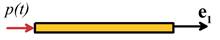A long thin rod occupies the region $x_1>0$, as shown in the figure.   It is made from a homogeneous, isotropic, linear elastic material with Young’s modulus E and mass density ${\rho }_0$.  At time t<0 it is at rest and free of stress.  At time t=0 it is subjected to a pressure p(t) at one end.  Calculate the displacement and stress fields in the solid.

 

We cheat by modeling this as a 1-D problem.  We assume that ${\sigma }_{11}$ is the only nonzero stress component, in which case the constitutive law and balance of linear momentum require that

$\begin{array}{l}{\sigma }_{11}=E{\displaystyle \frac{\partial u_1}{\partial x_1}{\displaystyle \frac{\partial {\sigma }_{11}}{\partial x_1}={\rho }_0{\displaystyle \frac{{\partial }^2{u}_1}{\partial t^2}}}}\\ \Rightarrow {\displaystyle \frac{{\partial }^2{u}_1}{\partial x_1{}^2}={\displaystyle \frac{1}{c_B^2}{\displaystyle \frac{{\partial }^2{u}_1}{\partial t^2}}}}\end{array}$

where $c_B^2=E/{\rho }_0$ is the wave speed. This equation is exact for $\nu =0$ but cannot be correct in general, since transverse motion is neglected.  In practice waves are repeatedly reflected off the sides of the bar, which behaves as a wave-guide (see Sect 5.6.5 for more discussion of wave-guides).

 

 It is straightforward to solve the equation to see that

$u_1(x_2,t)={\displaystyle \frac{c_B}{E}{\displaystyle \underset{0}{\overset{t-x_1/c_B}{\int }}p(\tau )d\tau }}$

${\sigma }_{11}=-p(t-x_1/c_B)$

 

 

 

4.3.4 Plane waves in an infinite solid

 

A plane wave that travels in direction p at speed c has a displacement field of the form

$u_i=a_{i}f(ct-x_k{p}_k)$

where p is a unit vector.  Again, to visualize this motion, consider the special case

$u=\left\{\begin{array}{c}0ct<x_k{p}_k\\ u_i=a_i(ct-x_k{p}_k)/cct\ge x_k{p}_k\end{array}\right.$

In this solution, the wave has a planar front, with normal vector p.  The wave travels in direction p at speed c.  Ahead of the front, the solid is at rest.  Behind it, the solid has velocity a.  For $a\cdot p=0$ the particle velocity is perpendicular to the wave velocity.  For $a=\alpha p$ the particle velocity is parallel to the wave velocity.  These two cases are like the shear and longitudinal waves discussed in the preceding sections.

 

We seek plane wave solutions of the Cauchy-Navier equation of motion

$C_{ijkl}{\displaystyle \frac{{\partial }^2{u}_k}{\partial x_j\partial x_l}={\rho }_0{\displaystyle \frac{{\partial }^2{u}_i}{\partial t^2}}}$

Substituting a plane wave solution for u we see that

$A_{ik}{a}_{k}f(ct-x_j{p}_j)=\rho a_i{c}^{2}f(ct-x_j{p}_j)$

where

$A_{jk}=C_{ijkl}{p}_i{p}_l$

is a symmetric, positive definite tensor known as the `Acoustic Tensor.’  Plane wave solutions to the Cauchy-Navier equation must therefore satisfy

$(A_{ik}-{\rho }_0{c}^2{\delta }_{ik})a_k=0$

This requires

$\det (A_{ik}-{\rho }_0{c}^2{\delta }_{ik})=0$

Evidently for any wave propagation direction, there are three wave speeds, and three corresponding displacement directions, which follow from the eigenvalues and eigenvectors of $A_{ij}/{\rho }_0$  For the special case of an isotropic solid

$C_{ijkl}=\mu \left({\delta }_{il}{\delta }_{jk}+{\delta }_{ik}{\delta }_{jl}\right)+{\displaystyle \frac{2\mu \nu }{1-2\nu }{\delta }_{ij}{\delta }_{kl}}$

where $\mu$ is the shear modulus and $\nu$ is the Poisson’s ratio of the solid.  The acoustic tensor follows as

$A_{ik}=\mu p_l{p}_l{\delta }_{ik}+{\displaystyle \frac{\mu }{1-2\nu }{p}_i{p}_k}$

so that

$\left(\mu -{\rho }_0{c}^2\right)a_k+{\displaystyle \frac{\mu }{1-2\nu }{p}_i{a}_i{p}_k=0}$

By inspection, there are two eigenvectors that satisfy this equation

 

1.       $a_i{p}_i=0\Rightarrow c^2=c_2^2={\rho }_0/\mu$                         (Shear wave,  or S-wave)

 

2.       $a_i=\eta p_i\Rightarrow c^2=c_L^2=2\mu (1-\nu )/{\rho }_0(1-2\nu )$  (Longitudinal, or P-wave)

 

 

The two wave speeds are evidently those we found in our 1-D calculation earlier.  So there are two types of plane wave in an isotropic solid.  The S-wave travels at speed $c_s$, and material particles are displaced perpendicular to the direction of motion of the wave.  The P-wave travels at speed $c_L$, and material particles are displaced parallel to the direction of motion of the wave.

 

 

 

4.3.5: Summary of Wave Speeds in isotropic elastic solids.

 

It is worth summarizing the three wave speeds calculated in the preceding sections.  Recall that

                                                          $\begin{array}{l}{c}_L^2={\displaystyle \frac{E(1-\nu )}{{\rho }_0(1+\nu )(1-2\nu )}={\displaystyle \frac{2\mu (1-\nu )}{{\rho }_0(1-2\nu )}}}\\ c_s^2={\displaystyle \frac{E}{2(1+\nu ){\rho }_0}={\displaystyle \frac{\mu }{{\rho }_0}}}\\ c_B^2={\displaystyle \frac{E}{{\rho }_0}}\end{array}$

It is straightforward to show that, for all positive definite materials (those with positive definite strain energy density $–$ a thermodynamic constraint) $c_L>c_S$.  For most real materials $c_L>c_B>c_s$.

 

There are also special kinds of waves (called Rayleigh and Stoneley waves) that travel near the surface of a solid, or near the interface between two dissimilar solids, respectively.  These waves have their own speeds.  Rayleigh waves are discussed in more detail in Section 5.5.3.

 

 

 

4.3.6: Reflection of waves traveling normal to a free surface

 

Suppose that a longitudinal wave with stress state

$\begin{array}{l}{u}_1(x_1,t)=-{\displaystyle \frac{c_L}{E}{\displaystyle \frac{(1+\nu )(1-2\nu )}{(1-\nu )}{\displaystyle \underset{0}{\overset{t-x_2/c_L}{\int }}f(\tau )d\tau }}}\\ u_2=u_3=0\\ {\sigma }_{11}=f(t-x_1/c_L)\end{array}$

is incident on a free surface at $x_1=a$, as shown in the figure below.  Our objective is to calculate the state of stress in the solid as a function of time, accounting for the stress free surface.

 

To visualize the wave, imagine that it is a front, such as would be generated by applying a constant uniform pressure at $x_1=0$ at time t=0.  The material ahead of the front is at rest, and stress free, while behind the front material has a constant stress and velocity. 

 

At time $t=a/c_L$ the front would reach the free surface and be reflected.  Let the horizontal stress associated with the reflected wave be

${\sigma }_{11}=g(t+x_1/c_L)$

(we need a + in the argument because the wave travels to the left and has negative velocity). For the stress to vanish at the free surface, we must have

$f(t-a/c_L)+g(t+a/c_L)=0$

so,

$g(t+x_1/c_L)=-f(t-a/c_L+(x_1-a)/c_L)$

and the full solution consists of both incident and reflected waves

$\begin{array}{l}{u}_1(x_1,t)=-{\displaystyle \frac{c_L}{E}{\displaystyle \frac{(1+\nu )(1-2\nu )}{1-\nu }\left\{{\displaystyle \underset{0}{\overset{t-x_2/c_L}{\int }}f(\tau )d\tau }+{\displaystyle \underset{0}{\overset{t-a/c_L+(x_2-a)/c_L}{\int }}f(\tau )d\tau }\right\}}}\\ u_2=u_3=0\\ {\sigma }_{11}=f(t-x_1/c_L)-f(t-a/c_L+(x_1-a)/c_L)\end{array}$

 

As a specific example, consider a plane, constant-stress wave that is incident on a free surface. The histories of stress and velocity in the solid are illustrated below.  

 

 

 In this case:

 

1. Behind the incident stress wave, the stress is constant, with magnitude ${\sigma }_0$.   The velocity of the solid is constant, and related to the stress by $v_1=-{\sigma }_0/(\rho c_L)$

 

2. At time $t=a/c_L$ the stress wave reaches the free surface.  At this time an equal and opposite stress pulse $-{\sigma }_0$ is reflected from the free surface, and propagates away from the surface.

 

3. Behind the reflected wave, the solid is stress free, and, the solid has constant velocity  $v_1=-2{\sigma }_0/(\rho c_L)$

 

 

 

4.3.7: Reflection and Transmission of waves normal to an interface

 

The problem to be solved is illustrated in the figure.   The material on the left has mass density ${\rho }_0$ and elastic properties that give a longitudinal wave speed $c_L$.  The corresponding properties for the material on the right are ${\rho }_B,c_L^B$. Suppose that a longitudinal wave with displacement and stress state

$\begin{array}{l}{u}_1(x_1,t)=-{\displaystyle \frac{c_L}{E}{\displaystyle \frac{(1+\nu )(1-2\nu )}{(1-\nu )}{\displaystyle \underset{0}{\overset{t-x_2/c_L}{\int }}f(\tau )d\tau }}}\\ u_2=u_3=0\\ {\sigma }_{11}=f(t-x_1/c_L)\end{array}$

is incident on a bi-material interface at $x_1=a$.  Calculate the state of stress in the solid as a function of time, accounting for the interface.

 

As before, waves will be reflected at the bi-material interface.  This time, however, some of the energy will be reflected, while some will be transmitted into the adjacent solid.  Guided by the solution to the preceding problem, we assume that the stress associated with the reflected and transmitted waves have the form

$\begin{array}{l}{\sigma }_{11}=g(t-a/c_L+(x_1-a)/c_L)\\ {\sigma }_{11}=h(t-a/c_L-(x_1-a)/c_L^B)\end{array}$

The functions g and h must be chosen to satisfy stress and displacement continuity at the interface.  Thes are:

 

1. Stress continuity requires that

$f(t-a/c_L)+g(t-a/c_L)=h(t-a/c_L)$

 

2. To satisfy displacement continuity, we make the acceleration continuous

$\begin{array}{l}{\rho }_0{\displaystyle \frac{{\partial }^2{u}_1}{\partial t^2}={\displaystyle \frac{\partial {\sigma }_{11}}{\partial x_1}}}\\ \Rightarrow -{\displaystyle \frac{f\text{'}(t-a/c_L)}{{\rho }_0{c}_L}+{\displaystyle \frac{g\text{'}(t-a/c_L)}{{\rho }_0{c}_L}=-{\displaystyle \frac{h\text{'}(t-a/c_L^B)}{{\rho }_B{c}_L^B}}}}\end{array}$

which may be integrated to give

$-{\displaystyle \frac{f(t-a/c_L)}{{\rho }_0{c}_L}+{\displaystyle \frac{g(t-a/c_L)}{{\rho }_0{c}_L}=-{\displaystyle \frac{h(t-a/c_L^B)}{{\rho }_B{c}_L^B}+C}}}$   

where C is a constant of integration.  Setting t=0 shows that C must vanish, since f=g=h=0 at t=0.  

 

 

The two conditions (1) and (2) may now be solved for g and h to see that

 

Reflected wave     ${\sigma }_{11}^{(r)}={\beta }_{r}f(t-a/c_L+(x_1-a)/c_L)$

Transmitted wave ${\sigma }_{11}^{(t)}={\beta }_{t}f(t-a/c_L-(x_1-a)/c_L^B)$

 

where the coefficients of reflection and transmission are given by

${\beta }_r={\displaystyle \frac{{\rho }_B{c}_L^B-{\rho }_0{c}_L}{{\rho }_B{c}_L^B+{\rho }_0{c}_L}{\beta }_t={\displaystyle \frac{2{\rho }_B{c}_L^B}{{\rho }_B{c}_L^B+{\rho }_0{c}_L}}}$

Results for a shear wave approaching the interface follow immediately from the preceding calculation, by simply setting $c_L=c_s$.

 

 

 

4.3.8: Simple example involving plane wave propagation: the plate impact experiment

 

A plate impact experiment is used to measure the plastic properties of materials at high rates of strain.  In typical experiment, a large, elastic flyer plate is fired (e.g. by a gas-gun) at a stationary target plate.   The specimen is a thin film of material, which is usually deposited on the surface of the flyer plate.   When the flyer plate impacts the target, plane pressure and shear waves begin to propagate through both plates, as shown in the figure.  The experiment is designed so that the target and flier plates remain elastic, while the thin film specimen deforms plastically.   A laser interferometer is used to monitor the velocity of the back face of the target plate: these measurements enable the history of stress and strain in the film to be reconstructed.

 

A full analysis of the plate impact experiment will not be attempted here $–$ instead, we illustrate the general procedure for modeling plane wave propagation in the plate impact experiment using a simple example. Suppose that

 

· Two elastic plates with Young’s modulus E, Poisson’s ratio $\nu$ and density $\rho$ are caused to collide, as shown in the figure.

 

· As a representative example, we suppose that the target has thickness $h$, while the projectile has thickness $2h$, as shown. The thickness of both flyer and target are assumed to be much smaller than any other relevant dimension (so wave reflection off lateral boundaries can be neglected).

 

· For simplicity, we assume that the faces of flyer and target are perpendicular to the direction of motion.  This means that the particle velocity in both flyer and target remains perpendicular to their surfaces throughout.

 

· Just prior to impact, the projectile has a uniform velocity $v_0$, while the target is stationary.

 

· At impact, plane pressure waves are initiated at the impact surface and propagate (in opposite directions) through both target and projectile.  Our objective is to calculate the history of stress and velocitity in both plates.

 

The resulting stress and motion in the plate is most conveniently displayed on “(x-t) diagrams” as shown below.  The graphs can be used to deduce the velocity and stress in both flyer and target at any position x and time t in both plates.  The solution consists of triangular regions (of time and position) of constant velocity and stress, separated by lines with slope equal to the longitudinal wave speed $c_L$ in the two plates (these lines are called “characteristics”).  Note that the stress and velocity have constant discontinuities across each characteristic.

 

      

The figure illustrates the following sequence of events:

 

1. Just after impact, plane pressure waves propagate in opposite directions through the flyer and target.  Behind the traveling wave fronts, both plates have velocity $v_1=v_0/2$ and are subjected to a stress state ${\sigma }_{11}={\sigma }_{22}={\sigma }_{33}=-{\sigma }_0$, where ${\sigma }_0=v_0\rho c_L/2$.

 

2. At time $t=h/c_L$ the wave propagating in the target plate reaches the free surfaces on the back side of the target.  The wave is reflected from the free surface.  Behind this reflected wave, the target is stress free, and has velocity $v_0$.  The target thereafter continues to travel at constant speed and remains free of stress indefinitely.

 

3. At time $t=2h/c_L$ there are two simultaneous events: (i) the plane wave in the flyer is reflected off the back surface $–$ behind the reflected wave the flyer is stress free and has zero velocity; (ii) the reflected wave in the target reaches the interface.  Since the interface is in compression, and the stress merely drops to zero behind the reflected wave, it passes freely through the interface without reflection.

 

4. At time $t=3h/c_L$ the two reflected waves in the flyer meet at the mid-point of the flyer. Thereafter, the region between the two reflected waves in the flyer becomes tensile.  In addition, the flyer plate has speed $v_0/2$ between the two wavefronts.

 

5.  At time $t=4h/c_L$ the reflected wave from the back surface of the flyer reaches the interface.  The stress is tensile behind this wave front, and since the interface between flyer and target cannot support tension in behaves like a free surface, and the wave is reflected off the interface back into the flyer.  At the same time, the reflected wave from the target reaches the back face of the flyer and is reflected for a second time.

 

6. Thereafter, the target continues to propagate with constant velocity $v_0$, while the flyer contains two plane waves that are repeatedly reflected from its two surfaces.  These waves effectively cause the flyer to vibrate, while traveling with average speed $v_0/2$.

 

 

Derivation: The solution can be constructed using the simple 1-D solutions given in 4.3.1 and 4.3.6.  For example, to find the stress and velocity associated with the waves generated by the initial impact:

 

1. At the moment of impact, both flyer and target are subjected to a sudden pressure. Wave motion in both solids can  be analyzed using the solution given in 4.3.1.

 

2. Let $\Delta v_f$,  $\Delta v_t$ denote the change in velocity of the flyer and target, respectively, as a result of impact.

 

3. Let ${\sigma }_{11}={\sigma }_f$ and ${\sigma }_{11}={\sigma }_t$ denote the horizontal stress component behind the wavefronts in the target and flyer just after impact.

 

4. From Section 4.3.1 we know that the velocity change and stress are related by

$\Delta v_f=-{\sigma }_f/(\rho c_L)\Delta v_t=-{\sigma }_t/(\rho c_L)$

 

5. The target and flyer must have the same velocity at the impact surface.  Therefore $v_0-\Delta v_f=\Delta v_t$

 

6. The horizontal stress must be equal in both solids at the impact surface.  Therefore ${\sigma }_f={\sigma }_t$.

 

7. The four equations in steps 4-6 can be solved to yield $\Delta v_f=\Delta v_t=v_0/2$, ${\sigma }_f={\sigma }_t=-{\sigma }_0$, with ${\sigma }_0=v_0\rho c_L/2$.

 

 

The changes in stress and velocity that occur at each reflection can then be deduced using the results at the end of Section 4.3.6.  Alternatively the (x-t) diagrams can be constructed directly, by first drawing all the characteristic lines, and then deducing the velocity and stress in each sector of the diagram by noting that (i) the change in stress and velocity across each line must be constant; (ii) the overall momentum of the solid must be conserved, and (iii) the total energy of the solid must be conserved.