Chapter 5
Solutions for linear elastic solids

 

 

 

In the preceding chapter, we solved some simple linear elastic boundary value problems.  The problems were trivial, however, in that the stress, strain and displacement fields were axially or spherically symmetric.  Most problems of practical interest involve fully 3D stress and displamement fields.

 

It is extremely difficult to solve general boundary value problems.  However, some of the best mathematicians over the past 200 years have turned their attention to this matter, and have developed several very elegant techniques.  None of these are completely general, but solutions derived using these techniques have provided invaluable insight into the behavior of deformable solids. 

 

Sadly, these days any fool with a PC and a finite element package can solve virtually any linear elastic boundary value problem, so you will not be able to make a living calculating exact elasticity solutions.  Nevertheless, some exact solutions are of fundamental practical importance. Examples include contact problems, solutions for cracks, stress concentrations, thermal stress problems, and problems involving defects such as dislocations in solids.  It is worth seeing how such solutions were derived.

 

In addition, there are some very powerful theorems in linear elasticity (such as the principle of minimum potential energy, and the reciprocal theorem), which can be used to calculate quantities of interest without necessarily having to solve all the governing equations.

 

In this chapter, we present a very brief survey of the field of linear elasticity.  Specifically,

 

1. We will outline some important general features of solutions to boundary and initial value problems;

 

2. We will discuss some solution techniques and present solutions to selected boundary value problems of interest;

 

3. We will discuss energy methods for solving problems involving linear elastic solids, including the principle of minimum potential energy, the reciprocal theorem, and the Rayleigh-Ritz method for estimating natural frequencies of vibrating elastic solids.

 

 

 

 

5.1 General Principles

 

This section outlines briefly (and mostly without proofs!) the general principles that apply to solutions to all boundary value problems in static linear elasticity.

 

 

 

5.1.1 Summary of the governing equations of linear elasticity

 

Static problems. We already listed the governing equations of linear elasticity in our discussion of simple axisymmetric problems. They are repeated here for convenience.  

 

 

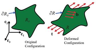
A representative problem is sketched above. We are given:

 

1. The shape of the solid in its unloaded condition $R_0\approx R$

 

2. The initial stress field in the solid (we will take this to be zero)

 

3. The elastic constants for the solid $C_{ijkl}$ and its mass density ${\rho }_0$

 

4. The thermal expansion coefficients for the solid, and temperature change from the initial configuration $\Delta T$

 

5. A body force distribution $b$ (per unit mass) acting on the solid

 

6. Boundary conditions, specifying displacements $u^{*}(x)$ on a portion ${\partial }_{1}R$ or tractions $t^{*}$ on a portion ${\partial }_{2}R$ of the boundary of R

 

 

We then seek to calculate displacements, strains and stresses satisfying the governing equations of linear elastostatics

$\begin{array}{l}{\epsilon }_{ij}={\displaystyle \frac{1}{2}\left({\displaystyle \frac{\partial u_i}{\partial x_j}+{\displaystyle \frac{\partial u_j}{\partial x_i}}}\right)}\\ {\sigma }_{ij}=C_{ijkl}({\epsilon }_{kl}-{\alpha }_{kl}\Delta T)\\ {\displaystyle \frac{\partial {\sigma }_{ij}}{\partial x_i}+{\rho }_0{b}_j=0}\\ u_i=u_i^{*}\text{on}{\partial }_{1}R\\ {\sigma }_{ij}{n}_i=t_j^{*}\text{on}{\partial }_{2}R\end{array}$

 

 

Dynamic problems Dynamic problems are essentially identical, except that the boundary conditions must be specified as functions of time, and the initial displacement and velocity field must be specified.  In this case the governing equations are

$\begin{array}{l}{\epsilon }_{ij}={\displaystyle \frac{1}{2}\left({\displaystyle \frac{\partial u_i}{\partial x_j}+{\displaystyle \frac{\partial u_j}{\partial x_i}}}\right)}\\ {\sigma }_{ij}=C_{ijkl}({\epsilon }_{kl}-{\alpha }_{kl}\Delta T)\\ {\displaystyle \frac{\partial {\sigma }_{ij}}{\partial x_i}+{\rho }_0{b}_j={\rho }_0{\displaystyle \frac{{\partial }^2{u}_j}{\partial t^2}}}\\ u_i=u_i^{*}(t)\text{on}{\partial }_{1}R\\ {\sigma }_{ij}{n}_i=t_j^{*}(t)\text{on}{\partial }_{2}R\end{array}$

 

 

 

5.1.2 Alternative form of the governing equations $–$ the Navier equation

 

The governing equations can be simplified by eliminating stress and strain from the governing equations, and solving directly for the displacements.  In this case the linear momentum balance equation (in terms of displacement) reduces to

$C_{ijkl}{\displaystyle \frac{\partial }{\partial x_i}\left({\displaystyle \frac{\partial u_k}{\partial x_l}-{\alpha }_{kl}\Delta T}\right)+{\rho }_0{b}_j={\rho }_0{\displaystyle \frac{{\partial }^2{u}_j}{\partial t^2}}}$

For the special case of an isotropic solid with shear modulus $\mu$ and Poisson ratio $\nu$ and uniform temperature $\Delta T=0$ this equation reduces to

${\displaystyle \frac{1}{1-2\nu }{\displaystyle \frac{{\partial }^2{u}_k}{\partial x_k\partial x_i}+{\displaystyle \frac{{\partial }^2{u}_i}{\partial x_k\partial x_k}+{\rho }_0{\displaystyle \frac{b_i}{\mu }={\displaystyle \frac{{\rho }_0}{\mu }{\displaystyle \frac{{\partial }^2{u}_i}{\partial t^2}}}}}}}$

These are known as the Navier (or Cauchy-Navier) equations of elasticity.

 

The boundary conditions remain as given in the preceding section.

 

 

 

5.1.3 Superposition and linearity of solutions

 

The governing equations of elasticity are linear.  This has two important consequences:

 

1. The stresses, strains and displacements in a solid are directly proportional to the loads (or displacements) applied to the solid. 

 

2. If you can find two sets of displacements, strains and stresses that satisfy the governing equations, you can add them to create more solutions.

 

 

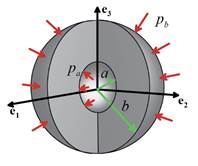
These principles can be illustrated clearly using some of the simple solutions derived in Section 4.1.  For example, examine the solution to the pressurized sphere illustrated in the figure (Sect 4.1.4).    As an example, the radial stress induced by pressure $p_a$ on the interior, and zero pressure on the exterior surface is

${\sigma }_{rr}={\displaystyle \frac{\left(p_a{a}^3\right)}{\left(b^3-a^3\right)}\left(1-{\displaystyle \frac{b^3}{r^2}}\right)}$    

The radial stress induced by pressure $p_b$ on the exterior surface, with zero pressure on the interior surface is

${\sigma }_{rr}=-{\displaystyle \frac{p_b{b}^3}{\left(b^3-a^3\right)}\left(1-{\displaystyle \frac{a^3}{r^3}}\right)}$

Note that in both cases the stress is directly proportional to the pressure.  In addition, to find the radial stress by combined pressures $p_a$ on the interior and $p_b$ on the exterior surface, you can just add these two solutions.

 

Further examples of superposition and linearity will be given in subsequent sections.

 

 

 

5.1.4 Uniqueness and existence of solutions to the linear elasticity equations

 

The following results are useful:

 

1. If only displacements are prescribed on the boundary of the solid, the governing equations of linear elasticity always have a solution, and the solution is unique.

 

2. If mixed boundary conditions are specified, a static solution exists and is unique if the displacements constrain rigid motions. A dynamic solution always exists and is unique, provided the velocity field and displacement field at time t=0 are known.

 

3. If only tractions are prescribed on the boundary, a static solution exists only if the tractions are in equilibrium.  In this case, the stresses and strains are unique, but the displacements are not.  A dynamic solution always exists and is unique, again, providing initial conditions are known.

 

 

 

 5.1.5 Saint-Venant’s principle

 

Saint-Venant’s principle is often invoked to formulate approximate solutions to boundary value problems in linear elasticity.  For example, when we solve problems involving bending or axial deformation of slender beams and rods in elementary strength of materials courses, we only specify the resultant forces acting on the ends of a rod, or the magnitudes of point forces acting on a beam, we don’t specify the distribution of traction in detail.  We rely on Saint Venant’s principle to justify this approach. In this context, the principle states the following.

 

The stresses, strains and displacements far from the ends of a rod or beam subjected to end loading depend only on the resultant forces and moments acting on its ends, and do not depend on how the tractions themselves are distributed.

 

Although SVP is widely used, it turns out to be remarkably difficult to prove mathematically.   The difficulty is partly that it is not easy to state the principle itself precisely enough to apply any mathematical machinery to it.  A rigorous statement is given by Sternberg (Q. J. Appl. Mech 11 p. 393 1954), among several other versions.  Here, we will just illustrate the most common applications of the principle through specific examples.

 

One version of SVP can be stated as follows.

 

Suppose that we calculate the stress, strain and displacement induced in a solid by two different traction distributions $t^{(1)}$ and $t^{(2)}$ that act on some small region of a solid with characteristic size a.  If the tractions exert the same resultant force and moment, then the stresses, strains and displacements induced by the two traction distributions at a distance r from the loaded region are identical for large $r/a$. 

 

In practice ‘large’ usually means $r/a>3$.

 

This principle can be illustrated using a simple example.

 

 

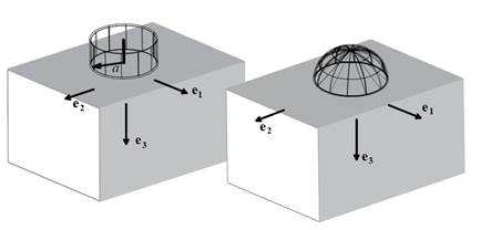
Consider a large solid with a flat surface, as shown above. It is possible to calculate formulas for the stresses and displacements induced by various pressure distributions acting on the flat surface $–$ the procedure to do this will be outlined later.  For now, we will compare the stresses induced by

 

1. A uniform pressure $p(r)=P/\left(\pi a^2\right)r\le a$

 

2. A parabolic pressure  $p(r)={\displaystyle \frac{3P}{2\pi a^2}{(1-r^2/a^2)}^{1/2}r\le a}$

 

 

You can verify for yourself that both pressure distributions exert a resultant force P acting in the vertical direction on the surface, and exert zero moment about the origin.  The variation of stress down the axis of symmetry ( $r=\sqrt{x_1^2+x_2^2}=0$ ), expressed in cylindrical-polar coordinates, can be derived as

 

Case 1: Uniform pressure

$\begin{array}{l}{\sigma }_{zz}=-{\displaystyle \frac{P}{\pi a^2}\left(1-{\displaystyle \frac{z_{}^3}{{(a^2+z^2)}^{3/2}}}\right)}\\ {\sigma }_{rr}={\sigma }_{\theta \theta }=-{\displaystyle \frac{P}{\pi a^2}\left({\displaystyle \frac{1+2\nu }{2}-{\displaystyle \frac{(1+\nu )z}{{(a^2+z^2)}^{1/2}}+{\displaystyle \frac{z^3}{2{(a^2+z^2)}^{3/2}}}}}\right)}\end{array}$

 

Case 2: Parabolic pressure

$\begin{array}{l}{\sigma }_{zz}=-{\displaystyle \frac{3P}{2\pi a^2}{\displaystyle \frac{a^2}{\left(a^2+z^2\right)}}}\\ {\sigma }_{rr}={\sigma }_{\theta \theta }=-{\displaystyle \frac{3P}{2\pi a^2}\left\{(1+\nu )\left(1-{\displaystyle \frac{z}{a}{\text{tan}}^{\text{-1}}{\displaystyle \frac{a}{z}}}\right)-{\displaystyle \frac{1}{2}{\displaystyle \frac{a^2}{a^2+z^2}}}\right\}}\end{array}$

 

Now, to demonstrate SVP, we want to show that the stresses are equal for large z/a.  We can do this graphically $–$ The figures compare the variation of vertical and radial stress down the axis of symmetry with z/a.

 

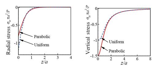
The stresses induced by the two different pressures are clearly indistinguishable for $z/a>3$.  This example helps to quantify what we mean by a `large’ distance.

 

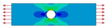
The second commonly used application of SVP is a rather vague statement that

 

 A localized geometrical feature with characteristic size R in a large solid only influences the stress in a region with size approximately 3R surrounding the feature.

 

This is more a rule of thumb than a precise mathematical statement.  It can be illustrated by looking at specific solutions.  For example, the figure below shows the von-Mises stress contours surrounding a circular hole in a thin rectangular plate that is subjected to extensional loading (calculated using the finite element method). Far from the hole, the stress is uniform.  The contours deviate from the uniform solution in a region that is about three times the hole radius.