5.2 Airy Function Solution to Plane Stress and Strain Static Linear Elastic Problems

 

In this section we outline a general technique for solving 2D static linear elasticity problems.  The technique is known as the `Airy Stress Function’ method.

 

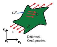A typical plane elasticity problem is illustrated in the figure. The solid is two dimensional, which means either that

 

1. The solid is a thin sheet, with small thickness h, and is loaded only in the $\{e_1,e_2\}$ plane.  In this case the plane stress solution is applicable

 

2. The solid is very long in the $e_3$ direction, is prevented from stretching parallel to the $e_3$ axis, and every cross section is loaded identically and only in the $\{e_1,e_2\}$ plane.  In this case, the plane strain solution is applicable.

 

 

Some additional basic assumptions and restrictions are:

 

· The Airy stress function is applicable only to isotropic solids.  We will assume that the solid has Young’s modulus E, Poisson’s ratio $\nu$ and mass density ${\rho }_0$

 

· The Airy Stress function can only be used if the body force has a special form. Specifically, the requirement is

${\rho }_0{b}_1={\displaystyle \frac{\partial \Omega }{\partial x_1}{\rho }_0{b}_2={\displaystyle \frac{\partial \Omega }{\partial x_2}{b}_3=0}}$

where $\Omega (x_1,x_2)$ is a scalar function of position.  Fortunately, most practical body forces can be expressed in this form, including gravity.

 

· The Airy Stress Function approach works best for problems where a solid is subjected to prescribed tractions on its boundary, rather than prescribed displacements.  Specifically, we will assume that the solid is loaded by boundary tractions $t_1(x_1,x_2)t_2(x_1,x_2)t_3=0$.

 

 

 

5.2.1 The Airy solution in rectangular coordinates

 

The Airy function procedure can then be summarized as follows:

 

1. Begin by finding a scalar function $\varphi (x_1,x_2)$ (known as the Airy potential) which satisfies:

${\nabla }^4\varphi \equiv {\displaystyle \frac{{\partial }^4\varphi }{\partial x_1^4}+2{\displaystyle \frac{{\partial }^4\varphi }{\partial x_1^2\partial x_2^2}+{\displaystyle \frac{{\partial }^4\varphi }{\partial x_1^4}=C\left(\nu \right){\rho }_0\left({\displaystyle \frac{\partial b_1}{\partial x_1}+{\displaystyle \frac{\partial b_2}{\partial x_2}}}\right)}}}$

where

$C\left(\nu \right)=\left\{\begin{array}{l}{\displaystyle \frac{1-\nu }{1-2\nu }\text{(Plane Strain)}}\\ {\displaystyle \frac{\text{1}}{\text{1}-\nu }\text{(Plane Stress)}}\end{array}\right.$

In addition, $\varphi$ must satisfy the following traction boundary conditions on the surface of the solid

${\displaystyle \frac{{\partial }^2\varphi }{\partial x_2^2}{n}_1-{\displaystyle \frac{{\partial }^2\varphi }{\partial x_1\partial x_2}{n}_2=t_1{\displaystyle \frac{{\partial }^2\varphi }{\partial x_1^2}{n}_2-{\displaystyle \frac{{\partial }^2\varphi }{\partial x_1\partial x_2}{n}_1=t_2}}}}$

where $(n_1,n_2)$ are the components of a unit vector normal to the boundary.

 

2. Given $\varphi$, the stress field within the region of interest can be calculated from the formulas

$\begin{array}{l}{\sigma }_{11}={\displaystyle \frac{{\partial }^2\varphi }{\partial x_2^2}-\Omega {\sigma }_{22}={\displaystyle \frac{{\partial }^2\varphi }{\partial x_1^2}-\Omega {\sigma }_{12}={\sigma }_{21}=-{\displaystyle \frac{{\partial }^2\varphi }{\partial x_1\partial x_2}}}}\\ {\sigma }_{33}=0(\text{Plane Stress)}\\ {\sigma }_{\text{33}}=\nu \left({\sigma }_{11}+{\sigma }_{22}\right)(\text{Plane Strain)}\\ {\sigma }_{\text{23}}={\sigma }_{13}=0\end{array}$

 

3. If the strains are needed, they may be computed from the stresses using the elastic stress$—$strain relations.

 

4. If the displacement field is needed, it may be computed by integrating the strains, following the procedure described in Section 2.2.15.  An example (in polar coordinates) is given in Section 5.2.4 below.

 

 

Although it is easier to solve for $\varphi$ than it is to solve for stress directly, this is still not a trivial exercise.  Usually, one guesses a suitable form for $\varphi$, as illustrated below.  This may seem highly unsatisfactory, but remember that we are essentially integrating a system of PDEs.  The general procedure to evaluate any integral is to guess a solution, differentiate it, and see if the guess was correct. 

 

 

 

5.2.2 Demonstration that the Airy solution satisfies the governing equations

 

Recall that to solve a linear elasticity problem, we need to satisfy the following equations:

 

· Displacement$—$strain relation ${\epsilon }_{ij}={\displaystyle \frac{1}{2}\left({\displaystyle \frac{\partial u_i}{\partial x_j}+{\displaystyle \frac{\partial u_j}{\partial x_i}}}\right)}$

 

· Stress$—$strain relation ${\epsilon }_{ij}={\displaystyle \frac{1+\nu }{E}{\sigma }_{ij}-{\displaystyle \frac{\nu }{E}{\sigma }_{kk}{\delta }_{ij}}}$

 

 

· Equilibrium Equation ${\displaystyle \frac{\partial {\sigma }_{ij}}{\partial x_i}+{\rho }_0{b}_j=0}$ 

 

where we have neglected thermal expansion, for simplicity.  We proceed to show that these equations are satisfied.

 

1. We show first that the Airy function satisfies the equilibrium equations automatically.  For plane stress or plane strain conditions, the equilibrium equations reduce to

${\displaystyle \frac{\partial {\sigma }_{11}}{\partial x_1}+{\displaystyle \frac{\partial {\sigma }_{12}}{\partial x_2}+{\rho }_0{b}_1=0{\displaystyle \frac{\partial {\sigma }_{12}}{\partial x_1}+{\displaystyle \frac{\partial {\sigma }_{22}}{\partial x_2}+{\rho }_0{b}_2=0}}}}$

Substitute for the stresses in terms of $\varphi$ to see that

$\begin{array}{l}{\displaystyle \frac{\partial }{\partial x_1}\left({\displaystyle \frac{{\partial }^2\varphi }{\partial x_2^2}-\Omega }\right)+{\displaystyle \frac{\partial }{\partial x_2}\left(-{\displaystyle \frac{{\partial }^2\varphi }{\partial x_1\partial x_2}}\right)+{\rho }_0{b}_1=0}}\\ {\displaystyle \frac{\partial }{\partial x_1}\left(-{\displaystyle \frac{{\partial }^2\varphi }{\partial x_1\partial x^2}}\right)+{\displaystyle \frac{\partial }{\partial x_2}\left({\displaystyle \frac{{\partial }^2\varphi }{\partial x_1^2}-\Omega }\right)+{\rho }_0{b}_2=0}}\end{array}$

so that the equilibrium equations are satisfied automatically for any choice of $\varphi$.

 

2. To show that the strain-displacement equation and the strain-displacement equation are satisfied, we first compute the strains using the elastic stress-strain equations.  Recall that

${\sigma }_{33}=\beta \nu \left({\sigma }_{11}+{\sigma }_{22}\right)$

with $\beta =0$ for plane stress and $\beta =1$ for plane strain.  Hence

$\begin{array}{l}{\epsilon }_{ij}={\displaystyle \frac{1+\nu }{E}{\sigma }_{ij}-{\displaystyle \frac{\nu }{E}{\sigma }_{kk}{\delta }_{ij}}}\\ \Rightarrow {\epsilon }_{11}={\displaystyle \frac{1+\nu }{E}{\sigma }_{11}-{\displaystyle \frac{\nu }{E}\left(1+\beta \nu \right)\left({\sigma }_{11}+{\sigma }_{22}\right)}}\\ {\epsilon }_{22}={\displaystyle \frac{1+\nu }{E}{\sigma }_{22}-{\displaystyle \frac{\nu }{E}\left(1+\beta \nu \right)\left({\sigma }_{11}+{\sigma }_{22}\right)}}\\ {\epsilon }_{12}={\displaystyle \frac{1+\nu }{E}{\sigma }_{12}}\end{array}$

Next, recall that the strain$—$displacement relation is satisfied provided that the strains obey the compatibility conditions

$\begin{array}{l}{\displaystyle \frac{{\partial }^2{\epsilon }_{11}}{\partial x_2^2}+{\displaystyle \frac{{\partial }^2{\epsilon }_{22}}{\partial x_1^2}-2{\displaystyle \frac{{\partial }^2{\epsilon }_{12}}{\partial x_1\partial x_2}=0}}}\\ {\displaystyle \frac{{\partial }^2{\epsilon }_{11}}{\partial x_3^2}+{\displaystyle \frac{{\partial }^2{\epsilon }_{33}}{\partial x_1^2}-2{\displaystyle \frac{{\partial }^2{\epsilon }_{13}}{\partial x_1\partial x_3}=0}}}\\ {\displaystyle \frac{{\partial }^2{\epsilon }_{22}}{\partial x_3^2}+{\displaystyle \frac{{\partial }^2{\epsilon }_{33}}{\partial x_2^2}-2{\displaystyle \frac{{\partial }^2{\epsilon }_{23}}{\partial x_2\partial x_3}=0}}}\end{array}$  

   $\begin{array}{l}{\displaystyle \frac{{\partial }^2{\epsilon }_{11}}{\partial x_2^{}\partial x_3^{}}-{\displaystyle \frac{\partial }{\partial x_1}\left(-{\displaystyle \frac{\partial {\epsilon }_{23}}{\partial x_1^{}}+{\displaystyle \frac{\partial {\epsilon }_{31}}{\partial x_2^{}}+{\displaystyle \frac{\partial {\epsilon }_{12}}{\partial x_3^{}}}}}\right)=0}}\\ {\displaystyle \frac{{\partial }^2{\epsilon }_{22}}{\partial x_3^{}\partial x_1^{}}-{\displaystyle \frac{\partial }{\partial x_2}\left(-{\displaystyle \frac{\partial {\epsilon }_{31}}{\partial x_2^{}}+{\displaystyle \frac{\partial {\epsilon }_{12}}{\partial x_3^{}}+{\displaystyle \frac{\partial {\epsilon }_{23}}{\partial x_1^{}}}}}\right)=0}}\\ {\displaystyle \frac{{\partial }^2{\epsilon }_{33}}{\partial x_1^{}\partial x_2^{}}-{\displaystyle \frac{\partial }{\partial x_3}\left(-{\displaystyle \frac{\partial {\epsilon }_{12}}{\partial x_3^{}}+{\displaystyle \frac{\partial {\epsilon }_{23}}{\partial x_1^{}}+{\displaystyle \frac{\partial {\epsilon }_{31}}{\partial x_2^{}}}}}\right)=0}}\end{array}$

 

All but the first of these equations are satisfied automatically by any plane strain or plane stress field. We therefore need to show that the Airy representation satisfies the first equation.  To see this substitute into the first compatibility equation in terms of stress to see that

$\begin{array}{l}{\displaystyle \frac{1+\nu }{E}\left({\displaystyle \frac{{\partial }^2{\sigma }_{11}}{\partial x_2^2}+{\displaystyle \frac{{\partial }^2{\sigma }_{22}}{\partial x_1^2}}}\right)-{\displaystyle \frac{\nu }{E}\left(1+\beta \nu \right)\left({\displaystyle \frac{{\partial }^2}{\partial x_1^2}+{\displaystyle \frac{{\partial }^2}{\partial x_2^2}}}\right)\left({\sigma }_{11}+{\sigma }_{22}\right)}}\\ -2{\displaystyle \frac{1+\nu }{E}{\displaystyle \frac{{\partial }^2{\sigma }_{12}}{\partial x_1\partial x_2}=0}}\end{array}$

Finally, substitute into this horrible looking equation for stress in terms of $\varphi$ and rearrange to see that

$\begin{array}{l}{\displaystyle \frac{{\partial }^4\varphi }{\partial x_2^4}-{\displaystyle \frac{{\partial }^2\Omega }{\partial x_2^2}+{\displaystyle \frac{{\partial }^4\varphi }{\partial x_1^4}-{\displaystyle \frac{{\partial }^2\Omega }{\partial x_1^2}-{\displaystyle \frac{\nu \left(1+\beta \nu \right)}{1+\nu }\left({\displaystyle \frac{{\partial }^2}{\partial x_1^2}+{\displaystyle \frac{{\partial }^2}{\partial x_2^2}}}\right)\left({\displaystyle \frac{{\partial }^2\varphi }{\partial x_1^2}+{\displaystyle \frac{{\partial }^2\varphi }{\partial x_2^2}-2\Omega }}\right)}}}}}\\ +2{\displaystyle \frac{{\partial }^4\varphi }{\partial x_1^2\partial x_2^2}=0}\end{array}$

A few more weeks of algebra reduces this to

${\displaystyle \frac{{\partial }^4\varphi }{\partial x_1^4}+2{\displaystyle \frac{{\partial }^4\varphi }{\partial x_1^2\partial x_2^2}+{\displaystyle \frac{{\partial }^4\varphi }{\partial x_2^4}={\displaystyle \frac{1-\beta {\nu }^2}{1-\nu -2\beta {\nu }^2}\left({\displaystyle \frac{{\partial }^2\Omega }{\partial x_1^2}+{\displaystyle \frac{{\partial }^2\Omega }{\partial x_2^2}}}\right)}}}}$

This is the governing equation for the Airy function $–$ so if the governing equation is satisfied, then the compatibility equation is also satisfied.

 

 

This proves that the Airy representation satisfies the governing equations.  A second important question is $–$ is it possible to find an Airy function for all 2D plane stress and plane strain problems?  If not, the method would be useless, because you couldn’t tell ahead of time whether $\varphi$ existed for the problem you were trying to solve.  Fortunately, it is possible to prove that all properly posed 2D elasticity problems do have an Airy representation.

 

 

 

5.2.3 The Airy solution in cylindrical-polar coordinates

 

Boundary value problems involving cylindrical regions are best solved using Cylindrical-polar coordinates.  It is worth recording the Airy function equations for this coordinate system.

 

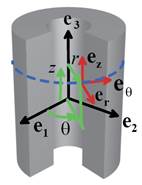
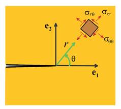
In a 2D cylindrical-polar coordinate system, a point in the solid is specified by its radial distance $r=\sqrt{x_1^2+x_2^2}$ from the origin and the angle $\theta ={\tan }^{-1}{x}_2/x_1$.  The solution is independent of z.  The Airy function is written as a function of the coordinates as $\varphi (r,\theta )$.  Vector quantities (displacement, body force) and tensor quantities (strain, stress) are expressed as components in the basis $\left\{e_r,e_{\theta },e_z\right\}$ shown in the figure.

 

The governing equation for the Airy function in this coordinate system is

$\begin{array}{c}{\left({\displaystyle \frac{{\partial }^2}{\partial r^2}+{\displaystyle \frac{1}{r}{\displaystyle \frac{\partial }{\partial r}+{\displaystyle \frac{1}{r^2}{\displaystyle \frac{{\partial }^2}{\partial {\theta }^2}}}}}}\right)}^2\varphi =C\left(\nu \right){\rho }_0\left({\displaystyle \frac{\partial b_r}{\partial r}+{\displaystyle \frac{1}{r}{\displaystyle \frac{\partial b_{\theta }}{\partial \theta }}}}\right)\\ C\left(\nu \right)=\left\{\begin{array}{l}{\displaystyle \frac{1-\nu }{1-2\nu }\text{(Plane Strain)}}\\ {\displaystyle \frac{\text{1}}{\text{1}-\nu }\text{(Plane Stress)}}\end{array}\right.\end{array}$

The state of stress is related to the Airy function by

$\begin{array}{l}{\sigma }_{rr}={\displaystyle \frac{1}{r}{\displaystyle \frac{\partial \varphi }{\partial r}+{\displaystyle \frac{1}{r^2}{\displaystyle \frac{{\partial }^2\varphi }{\partial {\theta }^2}-\Omega }}}}\\ {\sigma }_{\theta \theta }={\displaystyle \frac{{\partial }^2\varphi }{\partial r^2}-\Omega }\\ {\sigma }_{r\theta }=-{\displaystyle \frac{\partial }{\partial r}\left({\displaystyle \frac{1}{r}{\displaystyle \frac{\partial \varphi }{\partial \theta }}}\right)}\end{array}$

In polar coordinates the strains are related to the stresses by

$\left[\begin{array}{c}{\epsilon }_{rr}\\ {\epsilon }_{\theta \theta }\\ 2{\epsilon }_{r\theta }\end{array}\right]={\displaystyle \frac{(1+\nu )}{E}\left[\begin{array}{ccc}1-\nu & -\nu & 0\\ -\nu & 1-\nu & 0\\ 0& 0& 2\end{array}\right]\left[\begin{array}{c}{\sigma }_{rr}\\ {\sigma }_{\theta \theta }\\ {\sigma }_{r\theta }\end{array}\right]}$

for plane strain, while

$\left[\begin{array}{c}{\epsilon }_{rr}\\ {\epsilon }_{\theta \theta }\\ 2{\epsilon }_{r\theta }\end{array}\right]={\displaystyle \frac{1}{E}\left[\begin{array}{ccc}1& -\nu & 0\\ -\nu & 1& 0\\ 0& 0& 2(1+\nu )\end{array}\right]\left[\begin{array}{c}{\sigma }_{rr}\\ {\sigma }_{\theta \theta }\\ {\sigma }_{r\theta }\end{array}\right]}$

for plane stress.  The displacements must be determined by integrating these strains following the procedure similar to that outlined in Section 2.2.15.  To this end, let $u=u_r{e}_r+u_{\theta }{e}_{\theta }$ denote the displacement vector.  The strain-displacement relations in polar coordinates are:

$\begin{array}{l}{\epsilon }_{rr}={\displaystyle \frac{\partial u_r}{\partial r}}\\ {\epsilon }_{\theta \theta }={\displaystyle \frac{u_r}{r}+{\displaystyle \frac{1}{r}{\displaystyle \frac{\partial u_{\theta }}{\partial \theta }}}}\\ {\epsilon }_{r\theta }={\displaystyle \frac{1}{2}\left({\displaystyle \frac{1}{r}{\displaystyle \frac{\partial u_r}{\partial \theta }+{\displaystyle \frac{\partial u_{\theta }}{\partial r}-{\displaystyle \frac{u_{\theta }}{r}}}}}\right)}\end{array}$

These can be integrated using a procedure analogous to that outlined in Section 2.1.15.  An example is given in Section 5.2.5.

 

In the following sections, we give several examples of Airy function solutions to boundary value problems.

 

 

 

5.2.4 Airy function solution to the end loaded cantilever

 

Consider a cantilever beam, with length L, height 2a and out-of-plane thickness b, as shown below.

 

 

The beam is made from an isotropic linear elastic solid with Young’s modulus $E$ and Poisson ratio $\nu$. The top and bottom of the beam $x_2=\pm a$ are traction free, the left hand end is subjected to a resultant force P, and the right hand end is clamped.  Assume that b<<a, so that a state of plane stress is developed in the beam. An approximate solution to the stress in the beam can be calculated from the Airy function

$\varphi =-{\displaystyle \frac{3P}{4ab}{x}_1{x}_2+{\displaystyle \frac{P}{4a^{3}b}{x}_1{x}_2^3}}$

You can easily show that this function satisfies the governing equation for the Airy function. The stresses follow as

$\begin{array}{l}{\sigma }_{11}={\displaystyle \frac{{\partial }^2\varphi }{\partial x_2^2}-\Omega ={\displaystyle \frac{3P}{2a^{3}b}{x}_1{x}_2}}\\ {\sigma }_{22}={\displaystyle \frac{{\partial }^2\varphi }{\partial x_1^2}-\Omega =0}\\ {\sigma }_{12}={\sigma }_{21}=-{\displaystyle \frac{{\partial }^2\varphi }{\partial x_1\partial x_2}={\displaystyle \frac{3P}{4ab}\left(1-{\displaystyle \frac{x_2^2}{a^2}}\right)}}\end{array}$

 

To see that this solution satisfies the boundary conditions, note that

 

1. The top and bottom surfaces of the beam $x_2=\pm a$ are traction free ( ${\sigma }_{ij}{n}_i=0$ ).  Since the normal is in the $e_2$ direction on these surfaces, this requires that ${\sigma }_{22}={\sigma }_{21}=0$.  The stress field clearly satisfies this condition.

 

2. The plane stress assumption automatically satisfies boundary conditions on $x_3=\pm b/2$.

 

3. The traction boundary condition on the left hand end of the beam ( $x_1=0$ ) was not specified in detail: instead, we only required that the resultant of the traction acting on the surface is $-P{e}_2$.  The normal to the surface at the left hand end of the beam is in the $-e_1$ direction, so the traction vector is

$t_i={\sigma }_{ij}{n}_i=-{\sigma }_{12}{\delta }_{i2}=-{\displaystyle \frac{3P}{4ab}\left(1-{\displaystyle \frac{x_2^2}{a^2}}\right){\delta }_{i2}}$

The resultant force can be calculated by integrating the traction over the end of the beam:

$F_i=b{\displaystyle \underset{-a}{\overset{a}{\int }}-{\displaystyle \frac{3P}{4ab}\left(1-{\displaystyle \frac{x_2^2}{a^2}}\right){\delta }_{i2}d{x}_2}}=-P{\delta }_{i2}$

The stresses thus satisfy the boundary condition.  Note that by Saint-Venant’s principle, other distributions of traction with the same resultant will induce the same stresses sufficiently far ( $x_1>3a$ ) from the end of the beam.

 

4. The boundary conditions on the right hand end of the beam are not satisfied exactly.  The exact solution should satisfy both $u_1=0$ and $u_2=0$ on $x_1=L$.  The displacement field corresponding to the stress distribution was calculated in the example problem in Sect 2.1.20, where we found that

$\begin{array}{l}{u}_1={\displaystyle \frac{3P}{4E{a}^{3}b}{x}_1^2{x}_2-{\displaystyle \frac{P}{4E{a}^{3}b}(2+\nu )x_2^3+{\displaystyle \frac{3P}{2E{a}^{3}b}(1+\nu )a^2{x}_2-\omega x_2+c}}}\\ u_2=-\nu {\displaystyle \frac{3P}{4E{a}^{3}b}{x}_1{x}_2^2-{\displaystyle \frac{P}{4E{a}^{3}b}{x}_1^3+\omega x_1+d}}\end{array}$

where $c,d,\omega$ are constants that may be selected to satisfy the boundary condition as far as possible.  We can satisfy $u_1=0$ and $u_2=0$ at some, but not all, points on $x_1=L$.  The choice is arbitrary.  Usually the boundary condition is approximated by requiring $u_1=u_2=\partial u_2/\partial x_1=0$ at $x_1=L$, $x_2=0$.  This gives $c=0$, $d=-P{L}^3/2E{a}^{3}b$ and $\omega =3P{L}^2/4E{a}^{3}b$.   By Saint-Venant’s principle, applying other boundary conditions (including the exact boundary condition) will not influence the stresses and displacements sufficiently far from the end.

 

 

 

5.2.5 2D Line load acting perpendicular to the surface of an infinite solid

 

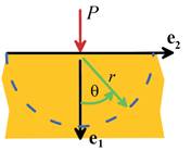As a second example, the stress fields due to a line load magnitude P per unit out-of-plane length acting on the surface of a homogeneous, isotropic half-space can be generated from the Airy function

$\varphi =-{\displaystyle \frac{P}{\pi }r\theta \sin \theta }$

where $(r,\theta )$ are cylindrical polar coordinates illustrated in the figure. The formulas in the preceding section yield

${\sigma }_{rr}=-{\displaystyle \frac{2P}{\pi }{\displaystyle \frac{\cos \theta }{r}{\sigma }_{\theta \theta }={\sigma }_{r\theta }=0}}$

 

The stresses in the $\{e_1,e_2,e_3\}$ basis are

${\sigma }_{11}=-{\displaystyle \frac{2P}{\pi }{\displaystyle \frac{x_1^3}{{\left(x_1^2+x_2^2\right)}^2}{\sigma }_{22}=-{\displaystyle \frac{2P}{\pi }{\displaystyle \frac{x_1^{}{x}_2^2}{{\left(x_1^2+x_2^2\right)}^2}{\sigma }_{12}=-{\displaystyle \frac{2P}{\pi }{\displaystyle \frac{x_1^2{x}_2^{}}{{\left(x_1^2+x_2^2\right)}^2}}}}}}}$

 

The method outlined in section 5.2.3 can be used to calculate the displacements: the procedure is described in detail below to provide a representative example.  For plane strain deformation, we find

$\begin{array}{l}{u}_r=-{\displaystyle \frac{2\left(1-{\nu }^2\right)}{\pi E}P\cos \theta \log r-{\displaystyle \frac{\left(1+\nu \right)\left(1-2\nu \right)}{\pi E}P\theta \sin \theta }}\\ u_{\theta }={\displaystyle \frac{2\left(1-{\nu }^2\right)}{\pi E}P\sin \theta \log r+{\displaystyle \frac{1+\nu }{\pi E}P\sin \theta -{\displaystyle \frac{2\left(1-2\nu \right)\left(1+\nu \right)}{\pi E}P\theta \cos \theta }}}\end{array}$

to within an arbitrary rigid motion.  Note that the displacements vary as log(r) so they are unbounded both at the origin and at infinity.  Moreover, the displacements due to any distribution of traction that exerts a nonzero resultant force on the surface will also be unbounded at infinity. 

 

It is easy to see that this solution satisfies all the relevant boundary conditions.  The surface is traction free ( ${\sigma }_{22}={\sigma }_{12}=0x_1=0$ ) except at r=0.  To see that the stresses are consistent with a vertical point force, note that the resultant vertical force exerted by the tractions acting on the dashed curve shown in the picture can be calculated as

$F_1={\displaystyle \underset{-\pi /2}{\overset{\pi /2}{\int }}{\sigma }_{rr}\cos \theta rd\theta }={\displaystyle \underset{-\pi /2}{\overset{\pi /2}{\int }}-{\displaystyle \frac{2P}{\pi }{\displaystyle \frac{\cos \theta }{r}\cos \theta rd\theta }}}=-P$

 

The expressions for displacement can be derived as follows.  Substituting the expression for stress into the stress-strain laws and using the strain-displacement relations yields

${\epsilon }_{rr}={\displaystyle \frac{\partial u_r}{\partial r}={\displaystyle \frac{\left(1+\nu \right)}{E}\left[(1-\nu ){\sigma }_{rr}-\nu {\sigma }_{\theta \theta }\right]=-{\displaystyle \frac{2P\left(1-{\nu }^2\right)}{\pi E}{\displaystyle \frac{\cos \theta }{r}}}}}$

Integrating

$u_r=-{\displaystyle \frac{2P\left(1-{\nu }^2\right)}{\pi E}\cos \theta \log (r)+f_r(\theta )}$

where $f_r(\theta )$ is a function of $\theta$ to be determined.  Similarly, considering the hoop stresses gives

${\epsilon }_{\theta \theta }={\displaystyle \frac{u_r}{r}+{\displaystyle \frac{1}{r}{\displaystyle \frac{\partial u_{\theta }}{\partial \theta }={\displaystyle \frac{\left(1+\nu \right)}{E}\left[(1-\nu ){\sigma }_{\theta \theta }-\nu {\sigma }_{rr}\right]={\displaystyle \frac{2P\nu (1+\nu )}{\pi E}{\displaystyle \frac{\cos \theta }{r}}}}}}}$

Rearrange and integrate with respect to $\theta$

$u_{\theta }={\displaystyle \frac{2P\left(1+\nu \right)}{\pi E}\sin \theta \left(\nu +(1-\nu )\log (r)\right)-{\displaystyle \int f_r(\theta )d\theta }+f_{\theta }(r)}$

where $f_{\theta }(r)$ is a function of $r$ to be determined.  Finally, substituting for stresses into the expression for shear strain shows that

${\epsilon }_{r\theta }={\displaystyle \frac{1}{2}\left({\displaystyle \frac{1}{r}{\displaystyle \frac{\partial u_r}{\partial \theta }+{\displaystyle \frac{\partial u_{\theta }}{\partial r}-{\displaystyle \frac{u_{\theta }}{r}}}}}\right)={\displaystyle \frac{\left(1+\nu \right)}{E}{\sigma }_{r\theta }=0}}$

Inserting the expressions for displacement and simplifying gives

${\displaystyle \frac{1}{r}\left\{{\displaystyle \frac{\partial f_r(\theta )}{\partial \theta }+{\displaystyle \int f_r(\theta )d\theta +{\displaystyle \frac{2P(1+\nu )(1-2\nu )}{\pi E}\sin \theta }}}\right\}+\left\{{\displaystyle \frac{\partial f_{\theta }(r)}{\partial r}-{\displaystyle \frac{f_{\theta }(r)}{r}}}\right\}=0}$

The two terms in parentheses are functions of $\theta$ and r, respectively, and so must both be separately equal to zero to satisfy this expression for all possible values of $\theta$ and r. Therefore

${\displaystyle \frac{{\partial }^2{f}_r(\theta )}{\partial {\theta }^2}+f_r(\theta )=-{\displaystyle \frac{2P(1+\nu )(1-2\nu )}{\pi E}\cos \theta }}$

This ODE has solution

$f_r(\theta )=-{\displaystyle \frac{P(1+\nu )(1-2\nu )}{\pi E}\theta \sin \theta +A\sin \theta +B\cos \theta }$

The second equation gives

${\displaystyle \frac{\partial f_{\theta }(r)}{\partial r}-{\displaystyle \frac{f_{\theta }(r)}{r}=0}}$

which has solution $f_{\theta }(r)=Cr$.  The constants A,B,C represent an arbitrary rigid displacement, and can be taken to be zero.  This gives the required answer.

 

 

 

5.2.6 2D Line load acting parallel to the surface of an infinite solid

 

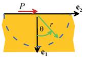Similarly, the stress fields due to a line load magnitude P per unit out-of-plane length acting tangent to the surface of a homogeneous, isotropic half-space can be generated from the Airy function

$\varphi =-{\displaystyle \frac{P}{\pi }r\theta \cos \theta }$

The formulas in the preceding section yield

${\sigma }_{rr}=-{\displaystyle \frac{2P}{\pi }{\displaystyle \frac{\sin \theta }{r}{\sigma }_{\theta \theta }={\sigma }_{r\theta }=0}}$

The method outlined in the preceding section can be used to calculate the displacements. The procedure gives

$\begin{array}{l}{u}_r=-{\displaystyle \frac{2\left(1-{\nu }^2\right)}{\pi E}P\sin \theta \log r-{\displaystyle \frac{\left(1+\nu \right)\left(1-2\nu \right)}{\pi E}P\theta \cos \theta }}\\ u_{\theta }={\displaystyle \frac{2\left(1-{\nu }^2\right)}{\pi E}P\cos \theta \log r+{\displaystyle \frac{1+\nu }{\pi E}P\cos \theta -{\displaystyle \frac{2\left(1-2\nu \right)\left(1+\nu \right)}{\pi E}P\theta \sin \theta }}}\end{array}$

to within an arbitrary rigid motion. 

 

The stresses and displacements in the $\{e_1,e_2,e_3\}$ basis are

${\sigma }_{11}=-{\displaystyle \frac{2P}{\pi }{\displaystyle \frac{x_1^2{x}_2}{{\left(x_1^2+x_2^2\right)}^2}{\sigma }_{22}=-{\displaystyle \frac{2P}{\pi }{\displaystyle \frac{x_2^3}{{\left(x_1^2+x_2^2\right)}^2}{\sigma }_{12}=-{\displaystyle \frac{2P}{\pi }{\displaystyle \frac{x_1^{}{x}_2^2}{{\left(x_1^2+x_2^2\right)}^2}}}}}}}$

 

 

 

5.2.7 Arbitrary pressure acting on a flat surface

 

The principle of superposition can be used to extend the point force solutions to arbitrary pressures acting on a surface. For example, we can find the solution for a uniform pressure acting on the strip of width 2a on the surface of a half-space by distributing the point force solution appropriately.  The figure illustrates the problem to be solved.

 

 

Distributing point forces with magnitude $p(s)ds{e}_1+q(s)ds{e}_2$ over the loaded region shows that

 

$\begin{array}{l}{\sigma }_{11}=-{\displaystyle \frac{2}{\pi }{\displaystyle \underset{A}{\int }{\displaystyle \frac{x_1^2(x_1^{}p(s)+\left(x_2-s\right)q(s))}{{\left(x_1^2+{\left(x_2-s\right)}^2\right)}^2}}}ds}\\ {\sigma }_{22}=-{\displaystyle \frac{2}{\pi }{\displaystyle \underset{A}{\int }{\displaystyle \frac{{(x_2-s)}^2\left(x_1^{}p(s)+(x_2-s)q(s)\right)}{{\left(x_1^2+{\left(x_2-s\right)}^2\right)}^2}}}ds}\\ {\sigma }_{12}=-{\displaystyle \frac{2}{\pi }{\displaystyle \underset{A}{\int }{\displaystyle \frac{x_1^{}(x_2^{}-s)\left(x_{1}p(s)+(x_2^{}-s)q(s)\right)}{{\left(x_1^2+{\left(x_2-s\right)}^2\right)}^2}ds}}}\end{array}$

 

 

 

5.2.8 Uniform normal pressure acting on a strip

 

For the particular case of a uniform pressure, the integrals can be evaluated to show that

$\begin{array}{l}{\sigma }_{22}=-{\displaystyle \frac{p}{2\pi }\left(2\left({\theta }_1-{\theta }_2\right)+\left(\sin 2{\theta }_1-\sin 2{\theta }_2\right)\right)}\\ {\sigma }_{11}=-{\displaystyle \frac{p}{2\pi }\left(2\left({\theta }_1-{\theta }_2\right)-\left(\sin 2{\theta }_1-\sin 2{\theta }_2\right)\right)}\\ {\sigma }_{12}={\displaystyle \frac{p}{2\pi }\left(\cos 2{\theta }_1-\cos 2{\theta }_2\right)}\end{array}$

where $0\le {\theta }_{\alpha }\le \pi$ and ${\theta }_1={\tan }^{-1}{x}_1/(x_2-a)$ ${\theta }_2={\tan }^{-1}{x}_1/(x_2+a)$ as shown below.

 

 

 

 

5.2.9 Stresses near the tip of a crack

 

Consider an infinite solid, which contains a semi-infinite crack on the (x1,x3) plane, as illustrated below

 

 

Suppose that the solid deforms in plane strain and is subjected to bounded stress at infinity.  The stress field near the tip of the crack can be derived from the Airy function

$\begin{array}{l}\varphi ={\displaystyle \frac{K_I}{3\sqrt{2\pi }}{r}^{3/2}\left(\cos 3\theta /2+3\cos \theta /2\right)}\\ -{\displaystyle \frac{K_{II}}{\sqrt{2\pi }}{r}^{3/2}\left(\sin 3\theta /2+\sin \theta /2\right)}\end{array}$

Here, $K_I$ and $K_{II}$ are two constants, known as mode I and mode II stress intensity factors, respectively.  They quantify the magnitudes of the stresses near the crack tip, as shown below. Their role will be discussed in more detail when we discuss fracture mechanics in Chapter 9. The stresses can be calculated as

$\begin{array}{l}{\sigma }_{rr}={\displaystyle \frac{K_I}{\sqrt{2\pi r}}\left({\displaystyle \frac{5}{4}\cos {\displaystyle \frac{\theta }{2}-{\displaystyle \frac{1}{4}\cos {\displaystyle \frac{3\theta }{2}}}}}\right)+{\displaystyle \frac{K_{II}}{\sqrt{2\pi r}}\left(-{\displaystyle \frac{5}{4}\sin {\displaystyle \frac{\theta }{2}+{\displaystyle \frac{3}{4}\sin {\displaystyle \frac{3\theta }{2}}}}}\right)}}\\ {\sigma }_{\theta \theta }={\displaystyle \frac{K_I}{\sqrt{2\pi r}}\left({\displaystyle \frac{3}{4}\cos {\displaystyle \frac{\theta }{2}+{\displaystyle \frac{1}{4}\cos {\displaystyle \frac{3\theta }{2}}}}}\right)-{\displaystyle \frac{K_{II}}{\sqrt{2\pi r}}\left({\displaystyle \frac{3}{4}\sin {\displaystyle \frac{\theta }{2}+{\displaystyle \frac{3}{4}\sin {\displaystyle \frac{3\theta }{2}}}}}\right)}}\\ {\sigma }_{r\theta }={\displaystyle \frac{K_I}{\sqrt{2\pi r}}\left({\displaystyle \frac{1}{4}\sin {\displaystyle \frac{\theta }{2}+{\displaystyle \frac{1}{4}\sin {\displaystyle \frac{3\theta }{2}}}}}\right)+{\displaystyle \frac{K_{II}}{\sqrt{2\pi r}}\left({\displaystyle \frac{1}{4}\cos {\displaystyle \frac{\theta }{2}+{\displaystyle \frac{3}{4}\cos {\displaystyle \frac{3\theta }{2}}}}}\right)}}\end{array}$

Equivalent expressions in rectangular coordinates are

$\begin{array}{l}{\sigma }_{11}={\displaystyle \frac{K_I}{\sqrt{2\pi r}}\cos {\displaystyle \frac{\theta }{2}\left(1-\sin {\displaystyle \frac{\theta }{2}\sin {\displaystyle \frac{3\theta }{2}}}\right)-{\displaystyle \frac{K_{II}}{\sqrt{2\pi r}}\sin {\displaystyle \frac{\theta }{2}\left(2+\cos {\displaystyle \frac{\theta }{2}\cos {\displaystyle \frac{3\theta }{2}}}\right)}}}}\\ {\sigma }_{22}={\displaystyle \frac{K_I}{\sqrt{2\pi r}}\cos {\displaystyle \frac{\theta }{2}\left(1+\sin {\displaystyle \frac{\theta }{2}\sin {\displaystyle \frac{3\theta }{2}}}\right)+{\displaystyle \frac{K_{II}}{\sqrt{2\pi r}}\cos {\displaystyle \frac{\theta }{2}\sin {\displaystyle \frac{\theta }{2}\cos {\displaystyle \frac{3\theta }{2}}}}}}}\\ {\sigma }_{12}={\displaystyle \frac{K_I}{\sqrt{2\pi r}}\cos {\displaystyle \frac{\theta }{2}\sin {\displaystyle \frac{\theta }{2}\cos {\displaystyle \frac{3\theta }{2}+{\displaystyle \frac{K_{II}}{\sqrt{2\pi r}}\cos {\displaystyle \frac{\theta }{2}\left(1-\sin {\displaystyle \frac{\theta }{2}\sin {\displaystyle \frac{3\theta }{2}}}\right)}}}}}}\end{array}$

while the displacements can be calculated by integrating the strains, with the result

$\begin{array}{l}{u}_1={\displaystyle \frac{K_I}{\mu }\sqrt{{\displaystyle \frac{r}{2\pi }}}\left[1-2\nu +{\sin }^2{\displaystyle \frac{\theta }{2}}\right]\cos {\displaystyle \frac{\theta }{2}+{\displaystyle \frac{K_{II}}{\mu }\sqrt{{\displaystyle \frac{r}{2\pi }}}\left[2-2\nu +{\cos }^2{\displaystyle \frac{\theta }{2}}\right]\sin {\displaystyle \frac{\theta }{2}}}}}\\ u_2={\displaystyle \frac{K_I}{\mu }\sqrt{{\displaystyle \frac{r}{2\pi }}}\left[2-2\nu -{\cos }^2{\displaystyle \frac{\theta }{2}}\right]\sin {\displaystyle \frac{\theta }{2}+{\displaystyle \frac{K_{II}}{\mu }\sqrt{{\displaystyle \frac{r}{2\pi }}}\left[-1+2\nu +{\sin }^2{\displaystyle \frac{\theta }{2}}\right]\cos {\displaystyle \frac{\theta }{2}}}}}\end{array}$

Note that this displacement field is valid for plane strain deformation only.

 

Observe that the stress intensity factor has the bizarre units of $N{m}^{-3/2}$.