5.3 Complex Variable Solution to Plane Strain Static Linear Elastic Problems

 

Airy functions have been used to find many useful solutions to plane elastostatic boundary value problems.  The method does have some limitations, however.  The biharmonic equation is not the easiest field equation to solve, for one thing. Another limitation is that displacement components are difficult to determine from Airy functions, so that the method is not well suited to displacement boundary value problems.

 

In this section we outline a more versatile representation for 2D static linear elasticity problems, based on complex potentials.  The main goal is to provide you with enough background to be able to interpret solutions that use the complex variable formulation.  The techniques to derive the complex potentials are beyond the scope of this book, but can be found in most linear elasticity texts.

 

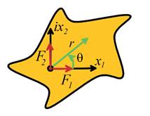
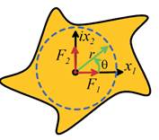
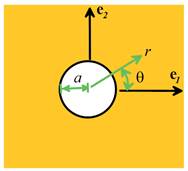
A typical plane elasticity problem is illustrated in the figure. Just as in the preceding section, we assume that the solid is two dimensional, which means either that

 

1. The solid is a thin sheet, with small thickness h, and is loaded only in the $\{e_1,e_2\}$ plane.  In this case the plane stress solution is applicable

 

2. The solid is very long in the $e_3$ direction, is prevented from stretching parallel to the $e_3$ axis, and every cross section is loaded identically and only in the $\{e_1,e_2\}$ plane.  In this case, the plane strain solution is applicable.

 

 

Some additional basic assumptions and restrictions are:

 

· The complex variable method outlined below is applicable only to isotropic solids.  We will assume that the solid has Young’s modulus E, Poisson’s ratio $\nu$ and mass density ${\rho }_0$

 

· We will assume no body forces, and constant temperature

 

 

 

5.3.1 Complex variable solutions to elasticity problems

 

The figure shows a 2D solid.  In the complex variable formalism,

 

· The position of a point in the solid is specified by a complex number $z=x_1+i{x}_2$

 

· The position of a point can also be expressed as $z=r{e}^{i\theta }$ where $r=\sqrt{x_1^2+x_2^2}\theta ={\tan }^{-1}{x}_2/x_1$. You can show that these are equivalent using Euler’s formula $e^{i\theta }=\cos \theta +i\sin \theta$, which gives

$\begin{array}{l}z=r{e}^{i\theta }=\sqrt{x_1^2+x_2^2}\left(\cos \theta +i\sin \theta \right)\\ =\sqrt{x_1^2+x_2^2}\left({\displaystyle \frac{x_1}{\sqrt{x_1^2+x_2^2}}+{\displaystyle \frac{i{x}_2}{\sqrt{x_1^2+x_2^2}}}}\right)\\ =x_1+i{x}_2\end{array}$

 

· The displacement of a point is specified using a second complex number $D=u_1+i{u}_2$

 

· The displacement and stress fields in rectangular coordinates are generated from two complex potentials $\Omega (z)$ and $\omega (z)$, which are differentiable (also called `analytic’ or `holomorphic’) functions of z  (e.g. a polynomial), using the following formulas

${\displaystyle \frac{E}{(1+\nu )}D=(3-4\nu )\Omega (z)-z\overline{{\Omega }^{\prime }(z)}-\overline{\omega (z)}}$

$\begin{array}{l}{\sigma }_{11}+{\sigma }_{22}=2\left({\Omega }^{\prime }(z)+\overline{{\Omega }^{\prime }(z)}\right)\\ {\sigma }_{11}-{\sigma }_{22}+2i{\sigma }_{12}=-2\left(z\overline{{\Omega }^{″}(z)}+\overline{{\omega }^{\prime }(z)}\right)\end{array}$

Here, ${\Omega }^{\prime }(z)$ denotes the derivative of $\Omega (z)$ with respect to z, and $\overline{\Omega (z)}$ denotes the complex conjugate of $\Omega (z)$.  Recall that to calculate the complex conjugate of a complex number, you simply change the sign of its imaginary part, i.e. $\overline{a+ib}=a-ib$.

 

· The displacement and stress in polar coordinates can be derived as

${\displaystyle \frac{E}{(1+\nu )}\left(u_r+i{u}_{\theta }\right)=\left[(3-4\nu )\Omega (z)-z\overline{{\Omega }^{\prime }(z)}-\overline{\omega (z)}\right]e^{-i\theta }}$

$\begin{array}{l}{\sigma }_{rr}+{\sigma }_{\theta \theta }=2\left({\Omega }^{\prime }(z)+\overline{{\Omega }^{\prime }(z)}\right)\\ {\sigma }_{rr}-{\sigma }_{\theta \theta }+2i{\sigma }_{r\theta }=-2\left(z\overline{{\Omega }^{″}(z)}+\overline{{\omega }^{\prime }(z)}\right)e^{-2i\theta }\end{array}$

 

· The formulas given here for displacements and stresses are the most general representation, but other special formulas are sometimes used for particular problems.  For example, if the solid is a half-space in the region  $x_2\ge 0$ with a boundary at $x_2=0$ the solution can be generated from a single complex potential $\Omega (z)$, using the formulas

$2\mu D=(3-4\nu )\Omega (z)+\Omega (\overline{z})+(\overline{z}-z)\overline{{\Omega }^{\prime }(z)}$

$\begin{array}{l}{\sigma }_{11}+{\sigma }_{22}=2\left({\Omega }^{\prime }(z)+\overline{{\Omega }^{\prime }(z)}\right)\\ {\sigma }_{22}-i{\sigma }_{12}={\Omega }^{\prime }(z)-{\Omega }^{\prime }(\overline{z})+(z-\overline{z})\overline{{\Omega }^{″}(z)}\end{array}$

For example, you can use these formulas to calculate stresses from the potentials given in Sections 5.3.7-5.3.9.  The conventional representation gives the same results, of course.

 

 

 

5.3.2 Demonstration that the complex variable solution satisfies the governing equations

 

We need to show two things:

 

1.  That the displacement field satisfies the equilibrium equation (See sect 5.1.2)

${\displaystyle \frac{1}{1-2\nu }{\displaystyle \frac{{\partial }^2{u}_k}{\partial x_k\partial x_i}+{\displaystyle \frac{{\partial }^2{u}_i}{\partial x_k\partial x_k}=0}}}$

 

2.  That the stresses are related to the displacements by the elastic stress-strain equations

 

To do this, we need to review some basic results from the theory of complex variables.  Recall that we have set $z=x_1+i{x}_2$, so that a differentiable function $f(z)$ can be decomposed into real and imaginary parts, each of which are functions of $x_1,x_2$, as

$f(z)=v(x_1,x_2)+iw(x_1,x_2)=v\left({\displaystyle \frac{z+\overline{z}}{2},i{\displaystyle \frac{\overline{z}-z}{2}}}\right)+iw\left({\displaystyle \frac{z+\overline{z}}{2},i{\displaystyle \frac{\overline{z}-z}{2}}}\right)$

This shows that

${\displaystyle \frac{\partial }{\partial z}\equiv {\displaystyle \frac{1}{2}\left({\displaystyle \frac{\partial }{\partial x_1}-i{\displaystyle \frac{\partial }{\partial x_2}}}\right){\displaystyle \frac{\partial }{\partial \overline{z}}\equiv {\displaystyle \frac{1}{2}\left({\displaystyle \frac{\partial }{\partial x_1}+i{\displaystyle \frac{\partial }{\partial x_2}}}\right)}}}}$

Next, recall that if $f(z)$ is differentiable with respect to z, its real and imaginary parts must satisfy the Cauchy-Riemann equations

${\displaystyle \frac{\partial v}{\partial x_1}={\displaystyle \frac{\partial w}{\partial x_2}{\displaystyle \frac{\partial w}{\partial x_1}=-{\displaystyle \frac{\partial v}{\partial x_2}}}}}$

We can then show that the derivative of $f(z)$ with respect to $\overline{z}$ is zero, and similarly, the derivative of $\overline{f(z)}$ with respect to z is zero.  To see these, use the definitions and the Cauchy-Riemann equations

$\begin{array}{l}2{\displaystyle \frac{\partial f(z)}{\partial \overline{z}}=\left({\displaystyle \frac{\partial }{\partial x_1}+i{\displaystyle \frac{\partial }{\partial x_2}}}\right)(v+iw)={\displaystyle \frac{\partial v}{\partial x_1}-{\displaystyle \frac{\partial w}{\partial x_2}+i({\displaystyle \frac{\partial v}{\partial x_2}+{\displaystyle \frac{\partial w}{\partial x_1})=0}}}}}\\ 2{\displaystyle \frac{\partial \overline{f(z)}}{\partial z}=\left({\displaystyle \frac{\partial }{\partial x_1}-i{\displaystyle \frac{\partial }{\partial x_2}}}\right)(v-iw)={\displaystyle \frac{\partial v}{\partial x_1}-{\displaystyle \frac{\partial w}{\partial x_2}-i({\displaystyle \frac{\partial v}{\partial x_2}+{\displaystyle \frac{\partial w}{\partial x_1})=0}}}}}\end{array}$

 

We can now proceed with the proof.   The equilibrium equations for plane deformation reduce to

$\begin{array}{l}\left({\displaystyle \frac{{\partial }^2}{\partial x_1^2}+{\displaystyle \frac{{\partial }^2}{\partial x_2^2}}}\right)u_1+{\displaystyle \frac{1}{1-2\nu }{\displaystyle \frac{\partial }{\partial x_1^{}}\left({\displaystyle \frac{\partial u_1}{\partial x_1^{}}+{\displaystyle \frac{\partial u_2}{\partial x_2^{}}}}\right)=0}}\\ \left({\displaystyle \frac{{\partial }^2}{\partial x_1^2}+{\displaystyle \frac{{\partial }^2}{\partial x_2^2}}}\right)u_2+{\displaystyle \frac{1}{1-2\nu }{\displaystyle \frac{\partial }{\partial x_2^{}}\left({\displaystyle \frac{\partial u_1}{\partial x_1^{}}+{\displaystyle \frac{\partial u_2}{\partial x_2^{}}}}\right)=0}}\end{array}$

These equations can be written in a combined, complex, form as

$\left({\displaystyle \frac{{\partial }^2}{\partial x_1^2}+{\displaystyle \frac{{\partial }^2}{\partial x_2^2}}}\right)(u_1+i{u}_2)+{\displaystyle \frac{1}{1-2\nu }\left({\displaystyle \frac{\partial }{\partial x_1^{}}+i{\displaystyle \frac{\partial }{\partial x_2^{}}}}\right)\left({\displaystyle \frac{\partial u_1}{\partial x_1^{}}+{\displaystyle \frac{\partial u_2}{\partial x_2^{}}}}\right)=0}$

It is easy to show (simply substitute $D=u_1+i{u}_2$ and use the definitions of differentiation with respect to $z$ and $\overline{z}$ ) that this can be re-written as

$4{\displaystyle \frac{{\partial }^2}{\partial z\partial \overline{z}}D+{\displaystyle \frac{2}{1-2\nu }{\displaystyle \frac{\partial }{\partial \overline{z}}\left({\displaystyle \frac{\partial D}{\partial z}+{\displaystyle \frac{\partial \overline{D}}{\partial \overline{z}}}}\right)=0}}}$

Finally, substituting

$D={\displaystyle \frac{\left(1+\nu \right)}{E}\left\{(3-4\nu )\Omega (z)-z\overline{{\Omega }^{\prime }(z)}-\overline{\omega (z)}\right\}}$

and noting that $\partial \Omega /\partial \overline{z}=0$ and $\partial \overline{\Omega }/\partial z=\partial \overline{\omega }/\partial z=0$ shows that this equation is indeed satisfied.

 

To show that the stress-strain relations are satisfied, note that the stress-strain relations for plane strain deformation (Section 3.1.4) can be written as

$\begin{array}{l}{\sigma }_{11}+{\sigma }_{22}={\displaystyle \frac{E}{(1+\nu )(1-2\nu )}\left({\displaystyle \frac{\partial u_1}{\partial x_1}+{\displaystyle \frac{\partial u_2}{\partial x_2}}}\right)={\displaystyle \frac{E}{(1+\nu )(1-2\nu )}\left({\displaystyle \frac{\partial D}{\partial z}+{\displaystyle \frac{\partial \overline{D}}{\partial \overline{z}}}}\right)}}\\ {\sigma }_{11}-{\sigma }_{22}+2i{\sigma }_{12}={\displaystyle \frac{E}{(1+\nu )}\left({\displaystyle \frac{\partial }{\partial x_1}+i{\displaystyle \frac{\partial }{\partial x_2}}}\right)(u_1+i{u}_2)={\displaystyle \frac{2E}{(1+\nu )}{\displaystyle \frac{\partial D}{\partial \overline{z}}}}}\end{array}$

Substituting for D in terms of the complex potentials and evaluating the derivatives gives the required results.

 

 

 

5.3.3 Complex variable solution for a line force in an infinite solid (plane strain deformation)

 

The figure shows a line load with force per unit out of plane distance $F=F_1{e}_1+F_2{e}_2$ acting at the origin of a large (infinite) solid. The displacements and stresses are calculated from the complex potentials

$\Omega (z)=-{\displaystyle \frac{F_1+i{F}_2}{8\pi (1-\nu )}\log (z)\omega (z)={\displaystyle \frac{(3-4\nu )(F_1-i{F}_2)}{8\pi (1-\nu )}\log (z)}}$

 

The displacements can be calculated from these potentials as

$\begin{array}{l}{u}_1=-{\displaystyle \frac{(1+\nu )F_1}{8\pi E(1-\nu )}\left\{2(3-4\nu )\log (r)+\cos 2\theta \right\}-{\displaystyle \frac{(1+\nu )F_2}{8\pi E(1-\nu )}\sin 2\theta }}\\ u_2=-{\displaystyle \frac{(1+\nu )F_2}{8\pi E(1-\nu )}\left\{2(3-4\nu )\log (r)-\sin 2\theta \right\}+{\displaystyle \frac{(1+\nu )F_1}{8\pi E(1-\nu )}\cos 2\theta }}\end{array}$

 

$\begin{array}{l}{\sigma }_{rr}=-{\displaystyle \frac{3-2\nu }{4\pi (1-\nu )r}\left(F_1\cos \theta +F_2\sin \theta \right)}\\ {\sigma }_{\theta \theta }={\displaystyle \frac{(1-2\nu )}{4\pi (1-\nu )r}\left(F_1\cos \theta +F_2\sin \theta \right)}\\ {\sigma }_{r\theta }={\displaystyle \frac{(1-2\nu )}{4\pi (1-\nu )r}\left(F_1\sin \theta -F_2\cos \theta \right)}\end{array}$

 

$\begin{array}{l}{\sigma }_{11}=-{\displaystyle \frac{F_1\cos \theta }{4\pi (1-\nu )r}\left(1-2\nu +2{\cos }^2\theta \right)+{\displaystyle \frac{F_2\sin \theta }{4\pi (1-\nu )r}\left(1-2\nu -2{\cos }^2\theta \right)}}\\ {\sigma }_{22}=-{\displaystyle \frac{F_1\cos \theta }{4\pi (1-\nu )r}\left(1+2\nu -2{\cos }^2\theta \right)-{\displaystyle \frac{F_2\sin \theta }{4\pi (1-\nu )r}\left(3-2\nu -2{\cos }^2\theta \right)}}\\ {\sigma }_{12}=-{\displaystyle \frac{F_1\sin \theta }{4\pi (1-\nu )r}\left(1-2\nu +2{\cos }^2\theta \right)-{\displaystyle \frac{F_2\cos \theta }{4\pi (1-\nu )r}\left(3-2\nu -2{\cos }^2\theta \right)}}\end{array}$

 

We will work through the algebra required to calculate these formulae for displacement and stress as a representative example.  In practice a symbolic manipulation program makes the calculations painless.  To begin, note that

$\log (z)=\log (r{e}^{i\theta })=\log (r)+i\theta$

and

${\displaystyle \frac{d}{dz}(\log (z))={\displaystyle \frac{1}{z}}}$

The displacements are thus

$\begin{array}{l}{\displaystyle \frac{E}{(1+\nu )}D=(3-4\nu )\Omega (z)-\overline{\omega (z)}-z\overline{{\Omega }^{\prime }(z)}}\\ =-{\displaystyle \frac{(3-4\nu )}{8\pi (1-\nu )}\left(\left(F_1+i{F}_2\right)\log (z)+\overline{\left(F_1-i{F}_2\right)}\overline{\log (z)}\right)-{\displaystyle \frac{\overline{F_1+i{F}_2}}{8\pi (1-\nu )}{\displaystyle \frac{z}{\overline{z}}}}}\\ =-{\displaystyle \frac{2(3-4\nu )}{8\pi (1-\nu )}\left(F_1+i{F}_2\right)\log (r)-{\displaystyle \frac{\left(F_1-i{F}_2\right)}{8\pi (1-\nu )}{\displaystyle \frac{r{e}^{i\theta }}{r{e}^{-i\theta }}}}}\\ =-{\displaystyle \frac{2(3-4\nu )}{8\pi (1-\nu )}\left(F_1+i{F}_2\right)\log (r)-{\displaystyle \frac{\left(F_1-i{F}_2\right)}{8\pi (1-\nu )}{e}^{2i\theta }}}\end{array}$

Finally, using Euler’s formula and taking real and imaginary parts gives the answer listed earlier.  Similarly, the formulas for stress give

$\begin{array}{l}{\sigma }_{rr}+{\sigma }_{\theta \theta }=2\left({\Omega }^{\prime }(z)+\overline{{\Omega }^{\prime }(z)}\right)=-{\displaystyle \frac{1}{4\pi (1-\nu )}\left({\displaystyle \frac{F_1+i{F}_2}{z}+{\displaystyle \frac{F_1-i{F}_2}{\overline{z}}}}\right)}\\ =-{\displaystyle \frac{(F_1+i{F}_2)e^{-i\theta }+(F_1-i{F}_2)e^{i\theta }}{4\pi (1-\nu )r}}\\ {\sigma }_{rr}-{\sigma }_{\theta \theta }+2i{\sigma }_{r\theta }=-2\left(z\overline{{\Omega }^{″}(z)}+\overline{{\omega }^{\prime }(z)}\right)e^{-2i\theta }\\ =-{\displaystyle \frac{e^{-2i\theta }}{4\pi (1-\nu )}\left\{(F_1-i{F}_2){\displaystyle \frac{r{e}^{i\theta }}{r^2{e}^{-2i\theta }}+(3-4\nu )(F_1+i{F}_2){\displaystyle \frac{1}{r{e}^{-i\theta }}}}\right\}}\\ =-{\displaystyle \frac{1}{4\pi (1-\nu )r}\left\{(F_1-i{F}_2)e^{i\theta }+(3-4\nu )(F_1+i{F}_2)e^{-i\theta }\right\}}\end{array}$

Adding the two formulas for stress shows that

$2{\sigma }_{rr}+2i{\sigma }_{r\theta }=-{\displaystyle \frac{1}{4\pi (1-\nu )r}\left\{2(F_1-i{F}_2)e^{i\theta }+4(1-\nu )(F_1+i{F}_2)e^{-i\theta }\right\}}$

Using Euler’s formula and taking real and imaginary parts of this expression gives the formulas for ${\sigma }_{rr}$ and ${\sigma }_{r\theta }$

 

Finally, we need to verify that the stresses are consistent with a point force acting at the origin.  To do this, we can evaluate the resultant force exerted by tractions acting on a circle enclosing the point force, as shown in the figure. Since the solid is in static equilibrium, the total force acting on this circular region must sum to zero.  Recall that the resultant force exerted by stresses on an internal surface can be calculated as

$R={\displaystyle \underset{A}{\int }n\cdot \sigma dA}$

A unit normal to the circle is $n=\cos \theta e_1+\sin \theta e_2$; multiplying by the stress tensor (in the $\{e_1,e_2,e_3\}$ basis) gives

$\begin{array}{l}{R}_1={\displaystyle \underset{0}{\overset{2\pi }{\int }}\left({\sigma }_{11}\cos \theta +{\sigma }_{12}\sin \theta \right)}rd\theta \\ R_2={\displaystyle \underset{0}{\overset{2\pi }{\int }}\left({\sigma }_{22}\sin \theta +{\sigma }_{12}\cos \theta \right)}rd\theta \end{array}$

Evaluating the integrals shows that $R_1=-F_1{R}_2=-F_2$, so $R+F_1{e}_1+F_2{e}_2=0$ as required.

 

 

 

 

5.3.4 Complex variable solution for an edge dislocation in an infinite solid

 

A dislocation is an atomic-scale defect in a crystal.  The defect can be detected directly in high-resolution transmission electron microscope pictures, which can show the positions of individual atoms in a crystal.  The leftmost figure below shows a typical example (an edge dislocation in a step-graded thin film of AlGaAsSb, kindly provided by Prof. David Paine of Brown University).  The dislocation is not easy to see, but can be identified by describing a `burger’s circuit’ around the dislocation, as shown by the yellow line.  Each straight portion of the circuit connects nine atoms.   In a perfect crystal, the circuit would start and end at the same atom.  (Try this for yourself for any path that does not encircle the dislocation).  Since the blue curve encircles the dislocation, it does not start and end on the same atom.  The `Burger’s vector’ for the dislocation is the difference in position vector of the start and end atom, as shown in the picture.

 

 

A continuum model of a dislocation can be created using the procedure illustrated in the right-hand figure above. Take an elastic solid, and cut part-way through it.  The edge of the cut defines a dislocation line $\xi$.  Next, displace the two material surfaces created by the cut by the burger’s vector b, and fill in the (infinitesimal) gap. Note that (by convention) the burger’s vector specifies the displacement of a point at the end of the Burger’s circuit as seen by an observer who sits on the start of the circuit, as shown in the picture.

 

HEALTH WARNING: Some texts define the Burger’s vector to be the negative of the vector defined here $–$ that is to say, the vector pointing from the end of the circuit back to the start.

 

 A general Burger’s vector has three components $–$ the component $b_s=b\cdot \xi$ parallel to the dislocation line is known as the screw component of b, while the two remaining components $b_e=b-b_s\xi$ are known as the edge components of b. The stress field induced by the dislocation depends only on $\xi$ and b, and is independent of the cut that created it.

 

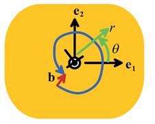
The figure above illustrates a pure edge dislocation, with line direction parallel to the $e_3$ axis and burgers vector $b=b_1{e}_1+b_2{e}_2$ at the origin of an infinite solid. The displacements and stresses can be derived from the complex potentials

$\Omega (z)=-i{\displaystyle \frac{E\left(b_1+i{b}_2\right)}{8\pi (1-{\nu }^2)}\log (z)\omega (z)=i{\displaystyle \frac{E(b_1-i{b}_2)}{8\pi (1-{\nu }^2)}\log (z)}}$

 

The displacement and stresses (in polar coordinates) can be derived from these potentials as

$\begin{array}{l}{u}_1={\displaystyle \frac{\theta b_1}{2\pi }+{\displaystyle \frac{1-2\nu }{4\pi (1-\nu )}{b}_2\log (r)-{\displaystyle \frac{1}{8\pi (1-\nu )}\left(b_2\cos 2\theta -b_1\sin 2\theta \right)}}}\\ u_2={\displaystyle \frac{\theta b_2}{2\pi }-{\displaystyle \frac{1-2\nu }{4\pi (1-\nu )}{b}_1\log (r)-{\displaystyle \frac{1}{8\pi (1-\nu )}\left(b_1\cos 2\theta +b_2\sin 2\theta \right)}}}\end{array}$

${\sigma }_{rr}={\sigma }_{\theta \theta }=-{\displaystyle \frac{E(b_1\sin \theta -b_2\cos \theta )}{4\pi (1-{\nu }^2)r}{\sigma }_{r\theta }={\displaystyle \frac{E(b_1\cos \theta +b_2\sin \theta )}{4\pi (1-{\nu }^2)r}}}$

$\begin{array}{l}{\sigma }_{11}=-{\displaystyle \frac{E{b}_1(3\sin \theta +\sin 3\theta )}{8\pi (1-{\nu }^2)r}+{\displaystyle \frac{E{b}_2(\cos \theta +\cos 3\theta )}{8\pi (1-{\nu }^2)r}}}\\ {\sigma }_{22}=-{\displaystyle \frac{E{b}_1(\sin \theta -\sin 3\theta )}{8\pi (1-{\nu }^2)r}+{\displaystyle \frac{E{b}_2(3\cos \theta -\cos 3\theta )}{8\pi (1-{\nu }^2)r}}}\\ {\sigma }_{12}=+{\displaystyle \frac{E{b}_1(\cos \theta +\cos 3\theta )}{8\pi (1-{\nu }^2)r}-{\displaystyle \frac{E{b}_2(\sin \theta -\sin 3\theta )}{8\pi (1-{\nu }^2)r}}}\end{array}$

 

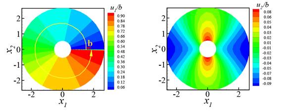
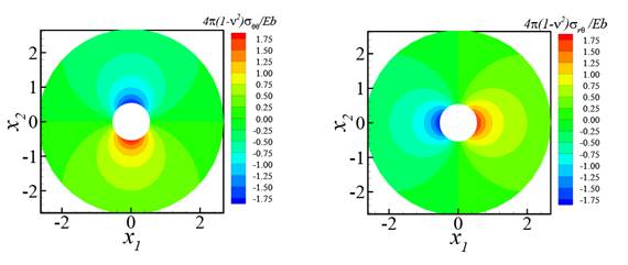
The displacement components are plotted below, for a dislocation with $b_2=0$.  The contours show a sudden jump in $u_1$ at $x_2=0,x_1>0$ (This is caused by the term involving $\theta$ in the formula for $u_1$ - we assumed that $0<\theta <2\pi$ when plotting the displacement contours). Physically, the plane $x_2=0,x_1>0$ corresponds to the `cut’ that created the dislocation, and the jump in displacement across the cut is equal to the Burger’s vector.

 

   

 

Contours of stress are plotted below.  The radial and hoop stresses are equal, and compressive above the dislocation, and tensile below it, as one would expect.  Shear stress is positive to the right of the dislocation and negative to the left, again, in concord with our physical intuition.  The stresses are infinite at the dislocation itself, but of course in this region linear elasticity does not accurately model material behavior, because the atomic bonds are very severely distorted.

 

 

 

 

5.3.5 Cylindrical hole in an infinite solid under remote loading

 

The figure shows a circular cylindrical cavity with radius a in an infinite, isotropic linear elastic solid. Far from the cavity, the solid is subjected to a tensile stress ${\sigma }_{11}={\sigma }_0$, with all other stress components zero.

 

 

The solution is generated by complex potentials

$\begin{array}{l}\Omega (z)={\displaystyle \frac{{\sigma }_0}{4}\left(z+{\displaystyle \frac{2a^2}{z}}\right)}\\ \omega (z)={\displaystyle \frac{-{\sigma }_0}{2}\left(z+{\displaystyle \frac{a^2}{z}-{\displaystyle \frac{a^4}{z^3}}}\right)}\end{array}$

 

The displacement and stress states are easily calculated as

$\begin{array}{l}{u}_1={\displaystyle \frac{{\sigma }_0(1+\nu )a}{2E}\left\{2\left(1-\nu \right)\left({\displaystyle \frac{r}{a}+{\displaystyle \frac{2a}{r}}}\right)\cos \theta +\left({\displaystyle \frac{a}{r}-{\displaystyle \frac{a^3}{r^3}}}\right)\cos 3\theta \right\}}\\ u_2={\displaystyle \frac{{\sigma }_0(1+\nu )a}{2E}\left\{-2\left(1-2\nu \right){\displaystyle \frac{a}{r}\sin \theta -2\nu {\displaystyle \frac{r}{a}\sin \theta +\left({\displaystyle \frac{a}{r}-{\displaystyle \frac{a^3}{r^3}}}\right)\sin 3\theta }}\right\}}\end{array}$

$\begin{array}{l}{\sigma }_{11}={\sigma }_0\left(1+\left({\displaystyle \frac{3a^4}{2r^4}-{\displaystyle \frac{a^2}{r^2}}}\right)\cos 4\theta -{\displaystyle \frac{3a^2}{2r^2}\cos 2\theta }\right)\\ {\sigma }_{22}={\sigma }_0\left(\left({\displaystyle \frac{a^2}{r^2}-{\displaystyle \frac{3a^4}{2r^4}}}\right)\cos 4\theta -{\displaystyle \frac{a^2}{2r^2}\cos 2\theta }\right)\\ {\sigma }_{12}={\sigma }_0\left(\left({\displaystyle \frac{3a^4}{2r^4}-{\displaystyle \frac{a^2}{r^2}}}\right)\sin 4\theta -{\displaystyle \frac{a^2}{2r^2}\sin 2\theta }\right)\end{array}$

 

 

 

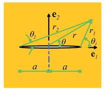
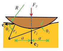
5.3.6 Crack in an infinite elastic solid under remote loading

 

The figure below shows a 2D crack with length 2a in an infinite solid, which is subjected to a uniform state of stress ${\sigma }_{22}^{\infty },{\sigma }_{12}^{\infty }$ at infinity. The solution can be generated by complex potentials

$\begin{array}{l}\Omega (z)={\displaystyle \frac{1}{4}\left({\sigma }_{22}^{\infty }\right)z+{\displaystyle \frac{1}{2}\left({\sigma }_{22}^{\infty }-i{\sigma }_{12}^{\infty }\right)\left(\sqrt{z^2-a^2}-z\right)}}\\ \omega (z)=\overline{\Omega (\overline{z})}-z{\Omega }^{\prime }(z)+{\sigma }_{22}^{\infty }z/2+i{\sigma }_{12}^{\infty }z\end{array}$

Here, the notation $\overline{\Omega (\overline{z})}$ indicates that you should substitute $\overline{z}$ into the function $\Omega$, and then take the conjugate of the whole function. Since $z$ gets conjugated twice, $\overline{\Omega (\overline{z})}$ is actually a function of $z$. It is an analytic function, and its derivative with respect to z can be calculated as $\overline{\Omega \text{'}(\overline{z})}$.

 

 

Some care is required to evaluate the square root in the complex potentials properly (square roots are multiple valued, and you need to know which value, or `branch’ to use.  Multiple valued functions are made single valued by introducing a `branch cut’ where the function is discontinuous.  In crack problems the branch cut is always along the line of the crack).  For this purpose, it is helpful to note that the appropriate branch can be obtained by setting

$\sqrt{z^2-a^2}=\sqrt{(z-a)(z+a)}=\sqrt{r_1}{e}^{i{\theta }_1/2}\sqrt{r_2}{e}^{i{\theta }_2/2}$

where the angles and distances $r_1,{\theta }_1$ and $r_2,{\theta }_2$ are shown above, and the angles ${\theta }_1$ and ${\theta }_2$ must lie in the ranges $-\pi \le {\theta }_1\le \pi 0\le {\theta }_2\le 2\pi$, respectively.

 

The solution is most conveniently expressed in terms of the polar coordinates $(r,\theta )$ centered at the origin, together with the auxiliary angles $r_1,{\theta }_1$ and $r_2,{\theta }_2$.  The displacement (for plane strain deformation) and stress fields are

$\begin{array}{l}{u}_1={\displaystyle \frac{1+\nu }{E}{\sigma }_{22}^{\infty }\sqrt{r_1{r}_2}\left\{(1-2\nu )\cos ({\theta }_1/2+{\theta }_2/2)-{\displaystyle \frac{r^2}{r_1{r}_2}\sin \theta \sin (\theta -{\theta }_1/2-{\theta }_2/2)}\right\}}\\ +{\displaystyle \frac{1+\nu }{E}{\sigma }_{12}^{\infty }\sqrt{r_1{r}_2}\left\{2(1+\nu )\sin ({\theta }_1/2+{\theta }_2/2)+{\displaystyle \frac{r^2}{r_1{r}_2}\sin \theta \cos (\theta -{\theta }_1/2-{\theta }_2/2)}\right\}}\end{array}$

$\begin{array}{l}{u}_2={\displaystyle \frac{1+\nu }{E}{\sigma }_{22}^{\infty }\sqrt{r_1{r}_2}\left\{2(1+\nu )\sin ({\theta }_1/2+{\theta }_2/2)-{\displaystyle \frac{r^2}{r_1{r}_2}\sin \theta \cos (\theta -{\theta }_1/2-{\theta }_2/2)}\right\}}\\ -{\displaystyle \frac{1+\nu }{E}{\sigma }_{12}^{\infty }\sqrt{r_1{r}_2}\left\{(1-2\nu )\cos ({\theta }_1/2+{\theta }_2/2)+{\displaystyle \frac{r^2}{r_1{r}_2}\sin \theta \sin (\theta -{\theta }_1/2-{\theta }_2/2)}\right\}}\end{array}$

 

$\begin{array}{l}{\sigma }_{11}={\displaystyle \frac{{\sigma }_{22}^{\infty }r}{\sqrt{r_1{r}_2}}\left\{\cos \left(\theta -{\theta }_1/2-{\theta }_2/2\right)-1-{\displaystyle \frac{a^2}{r_1{r}_2}\sin \theta \sin \left(3\left({\theta }_1+{\theta }_2\right)/2\right)}\right\}}\\ +{\displaystyle \frac{{\sigma }_{12}^{\infty }r}{\sqrt{r_1{r}_2}}\left\{2\sin \left(\theta -{\theta }_1/2-{\theta }_2/2\right)-{\displaystyle \frac{a^2}{r_1{r}_2}\sin \theta \cos \left(3\left({\theta }_1+{\theta }_2\right)/2\right)}\right\}}\\ {\sigma }_{22}={\displaystyle \frac{{\sigma }_{22}^{\infty }r}{\sqrt{r_1{r}_2}}\left\{\cos \left(\theta -{\theta }_1/2-{\theta }_2/2\right)+{\displaystyle \frac{a^2}{r_1{r}_2}\sin \theta \sin \left(3\left({\theta }_1+{\theta }_2\right)/2\right)}\right\}}\\ +{\displaystyle \frac{{\sigma }_{12}^{\infty }r}{\sqrt{r_1{r}_2}}{\displaystyle \frac{a^2}{r_1{r}_2}\sin \theta \cos \left(3\left({\theta }_1+{\theta }_2\right)/2\right)}}\\ {\sigma }_{12}={\displaystyle \frac{{\sigma }_{22}^{\infty }r}{\sqrt{r_1{r}_2}}{\displaystyle \frac{a^2}{r_1{r}_2}\sin \theta \cos \left(3\left({\theta }_1+{\theta }_2\right)/2\right)}}\\ +{\displaystyle \frac{{\sigma }_{12}^{\infty }r}{\sqrt{r_1{r}_2}}\left\{\cos \left(\theta -{\theta }_1/2-{\theta }_2/2\right)+{\displaystyle \frac{a^2}{r_1{r}_2}\sin \theta \sin \left(3\left({\theta }_1+{\theta }_2\right)/2\right)}\right\}}\end{array}$

 

 

 

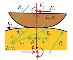
5.3.7 Fields near the tip of a crack on bimaterial interface

 

The figure shows a semi-infinite crack, which lies in the $x_1,x_3$ plane, with crack tip aligned with the $x_3$ axis.  The material above the crack has shear modulus and Poisson’s ratio ${\mu }_1,{\nu }_1$; the material below the crack has shear modulus and Poisson’s ratio ${\mu }_2,{\nu }_2$.  In this section we give the complex variable solution that governs the variation of stress and displacement near the crack tip.  The solution is significant because all interface cracks (regardless of their geometry and the way the solid is loaded) have the same stress and displacement distribution near the crack tip.

 

 

Additional elastic constants for bimaterial problems

 

To simplify the solution, we define additional elastic constants as follows

 

1. Plane strain moduli ${E^{\prime }}_1=2{\mu }_1/(1-{\nu }_1)$, ${E^{\prime }}_2=2{\mu }_2/(1-{\nu }_2)$

 

2. Bimaterial modulus ${\displaystyle \frac{1}{E^{*}}=\left\{{\displaystyle \frac{1}{{E^{\prime }}_1}+{\displaystyle \frac{1}{{E^{\prime }}_2}}}\right\}}$

 

 

3. Dundur’s elastic constants

$\alpha ={\displaystyle \frac{{E^{\prime }}_1-{E^{\prime }}_2}{{E^{\prime }}_1+{E^{\prime }}_2}\beta ={\displaystyle \frac{\left(1-2{\nu }_2\right)/{\mu }_2-\left(1-2{\nu }_1\right)/{\mu }_1}{2\left(1-{\nu }_2\right)/{\mu }_2+2\left(1-{\nu }_1\right)/{\mu }_1}}}$

Evidently $\alpha$ is a measure of the relative stiffness of the two materials.  It must lie in the range $-1<\alpha <1$ for all possible material combinations, with $\alpha =1$ signifying that material 1 is rigid, while $\alpha =-1$ signifies that material 2 is rigid.  The second parameter does not have such a nice physical interpretation $–$ it is a rough measure of the relative compressibilities of the two materials.  For Poisson’s ratios in the range $0<\nu <1/2$, one can show that that $-1<\alpha -4\beta <1$.

 

4. Crack tip singularity parameter

$\epsilon ={\displaystyle \frac{1}{2\pi }\log \left({\displaystyle \frac{1-\beta }{1+\beta }}\right)}$

For most material combinations the value of $\epsilon$ is very small $–$ typically of order 0.01 or so.

 

The full displacement and stress fields in the two materials are calculated from two sets of complex potentials

$\begin{array}{l}{\Omega }_1(z)={\displaystyle \frac{1+\beta }{(1-2i\epsilon )\sqrt{2\pi }}(K_1-i{K}_2)z^{(1-2i\epsilon )/2}\mathrm{Im}(z)>0}\\ {\Omega }_2(z)={\displaystyle \frac{1-\beta }{(1-2i\epsilon )\sqrt{2\pi }}(K_1-i{K}_2)z^{(1-2i\epsilon )/2}\mathrm{Im}(z)<0}\\ {\omega }_1(z)=\overline{{\Omega }_2(\overline{z})}-z{{\Omega }^{\prime }}_1(z)\mathrm{Im}(z)>0\\ {\omega }_2(z)=\overline{{\Omega }_1(\overline{z})}-z{{\Omega }^{\prime }}_2(z)\mathrm{Im}(z)<0\end{array}$

where $K_1$ and $K_2$ are parameters that resemble the mode I and mode II stress intensity factors that characterize the crack-tip stresses in a homogeneous solid.  In practice these parameters are not usually used in fracture criteria for interface cracks $–$ instead, the crack tip loading is characterized the magnitude of the stress intensity factor $\left|K\right|$, a characteristic length L, and a phase angle $\psi$, defined as

$\left|K\right|=\sqrt{K_1^2+K_2^2}\psi ={\tan }^{-1}{\displaystyle \frac{\mathrm{Im}\left[(K_1+i{K}_2)L^{i\epsilon }\right]}{\mathrm{Re}\left[(K_1+i{K}_2)L^{i\epsilon }\right]}}$

This means that $\left(K_1+i{K}_2\right)L^{i\epsilon }=\left|K\right|e^{i\psi }\Rightarrow \left(K_1-i{K}_2\right)=\left|K\right|e^{-i\psi }{L}^{i\epsilon }$.

 

Complete expressions for the displacement components and stress components at a point $r,\theta$ in the solid can be calculated from these potentials.  To simplify the results, it is helpful to note that

$\cosh (\pi \epsilon )={\displaystyle \frac{1}{2}\left(e^{\pi \epsilon }+e^{-\pi \epsilon }\right)={\displaystyle \frac{1}{2}\left(\sqrt{{\displaystyle \frac{1-\beta }{1+\beta }}}+\sqrt{{\displaystyle \frac{1+\beta }{1-\beta }}}\right)={\displaystyle \frac{1}{\sqrt{(1-\beta })\sqrt{(1+\beta )}}}}}$

Then, in material 1

$\begin{array}{l}2{\mu }_1(u_1+i{u}_2)={\displaystyle \frac{\left|K\right|}{\cosh (\pi \epsilon )}\sqrt{{\displaystyle \frac{r}{2\pi }}}\left\{{\displaystyle \frac{1}{1-2i\epsilon }{\left({\displaystyle \frac{r}{L}}\right)}^{-i\epsilon }\left[(3-4{\nu }_1)e^{i(\theta /2-\psi )}{e}^{\epsilon (\theta -\pi )}-e^{-i(\theta /2+\psi )}{e}^{-\epsilon (\theta -\pi )}\right]}\right.}\\ \left.-{\left({\displaystyle \frac{r}{L}}\right)}^{i\epsilon }i\sin \theta e^{i(\theta /2+\psi )}{e}^{\epsilon (\theta -\pi )}\right\}\end{array}$

$\begin{array}{l}{\sigma }_{11}+{\sigma }_{22}={\displaystyle \frac{\left|K\right|}{\sqrt{2\pi r}}\left(1+\beta \right)e^{\epsilon \theta }\left\{{\left({\displaystyle \frac{r}{L}}\right)}^{-i\epsilon }{e}^{-i(\theta /2+\psi )}+{\left({\displaystyle \frac{r}{L}}\right)}^{i\epsilon }{e}^{i(\theta /2+\psi )}\right\}}\\ {\sigma }_{11}-{\sigma }_{22}+2i{\sigma }_{12}={\displaystyle \frac{\left|K\right|e^{i\theta }}{\sqrt{2\pi r}}\left\{{\left({\displaystyle \frac{r}{L}}\right)}^{i\epsilon }{e}^{i\psi }{e}^{\epsilon \theta }{e}^{i\theta /2}\left(1+\beta \right)\left(\cos \theta +2\epsilon \sin \theta \right)\right.}\\ \left.-{\left({\displaystyle \frac{r}{L}}\right)}^{-i\epsilon }{e}^{-i\psi }{e}^{-\epsilon \theta }{e}^{-i\theta /2}\left(1-\beta \right)\right\}\end{array}$

while in material 2

$\begin{array}{l}2{\mu }_2(u_1+i{u}_2)={\displaystyle \frac{\left|K\right|}{\cosh (\pi \epsilon )}\sqrt{{\displaystyle \frac{r}{2\pi }}}\left\{{\displaystyle \frac{1}{1-2i\epsilon }{\left({\displaystyle \frac{r}{L}}\right)}^{-i\epsilon }\left[(3-4{\nu }_2)e^{i(\theta /2-\psi )}{e}^{\epsilon (\theta +\pi )}-e^{-i(\theta /2+\psi )}{e}^{-\epsilon (\theta +\pi )}\right]}\right.}\\ \left.-{\left({\displaystyle \frac{r}{L}}\right)}^{i\epsilon }i\sin \theta e^{i(\theta /2+\psi )}{e}^{\epsilon (\theta +\pi )}\right\}\end{array}$

$\begin{array}{l}{\sigma }_{11}+{\sigma }_{22}={\displaystyle \frac{\left|K\right|}{\sqrt{2\pi r}}\left(1-\beta \right)e^{\epsilon \theta }\left\{{\left({\displaystyle \frac{r}{L}}\right)}^{-i\epsilon }{e}^{-i(\theta /2+\psi )}+{\left({\displaystyle \frac{r}{L}}\right)}^{i\epsilon }{e}^{i(\theta /2+\psi )}\right\}}\\ {\sigma }_{11}-{\sigma }_{22}+2i{\sigma }_{12}={\displaystyle \frac{\left|K\right|e^{i\theta }}{\sqrt{2\pi r}}\left\{{\left({\displaystyle \frac{r}{L}}\right)}^{i\epsilon }{e}^{i\psi }{e}^{\epsilon \theta }{e}^{i\theta /2}\left(1-\beta \right)\left(\cos \theta +2\epsilon \sin \theta \right)\right.}\\ \left.-{\left({\displaystyle \frac{r}{L}}\right)}^{-i\epsilon }{e}^{-i\psi }{e}^{-\epsilon \theta }{e}^{-i\theta /2}\left(1+\beta \right)\right\}\end{array}$

The individual stress components can be determined by adding/subtracting the last two equations and taking real and imaginary parts.  Note that

${(r/L)}^{i\epsilon }=\exp (i\epsilon \log (r/L))=\cos (\epsilon \log (r/L))+i\sin (\epsilon \log (r/L))$.

Features of this solution are discussed in more detail in Section 9.6.1.

 

 

 

5.3.8 Frictionless rigid flat indenter in contact with a half-space

 

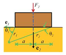The figure shows a rigid, flat punch with width 2a and infinite length perpendicular to the plane of the figure. It is pushed into an elastic half-space with a force $F_2$ per unit out of plane distance. The half-space is a linear elastic solid with shear modulus $\mu$ and Poisson’s ratio $\nu$. The interface between the two solids is frictionless. 

 

 

The solution is generated from the following complex potentials

$\begin{array}{l}\Omega (z)={\displaystyle \frac{-i{F}_2}{2\pi }\log \left(z+\sqrt{z^2-a^2}\right)+{\displaystyle \frac{\mu i{d}_2}{2(1-\nu )}}}\\ \omega (z)=-\overline{\Omega (\overline{z})}-z{\Omega }^{\prime }(z)\end{array}$

where $d_2$ is an arbitrary constant, representing an unknown rigid displacement. Note that the solution is valid only for $\mathrm{Im}(z)>0$.

 

Stresses and displacements can be determined by substituting for $\Omega$ and $\omega$ into the general formulas, or alternatively, by substituting $\Omega$ into the simplified representation for half-space problems given in 5.3.1. Some care is required to evaluate the square root in the complex potentials, particularly when calculating $\Omega (\overline{z})$ and ${\Omega }^{\prime }(\overline{z})$. The solution assumes that

$\begin{array}{l}\sqrt{z^2-a^2}=\sqrt{(z-a)(z+a)}=\sqrt{r_1}{e}^{i{\theta }_1/2}\sqrt{r_2}{e}^{i{\theta }_2/2}\\ \overline{\sqrt{z^2-a^2}}=\overline{\sqrt{(z-a)(z+a)}}=\sqrt{r_1}{e}^{-i{\theta }_1/2}\sqrt{r_2}{e}^{-i{\theta }_2/2}\\ \sqrt{{\overline{z}}^2-a^2}=\sqrt{(\overline{z}-a)(\overline{z}+a)}=\sqrt{r_1}{e}^{-i{\theta }_1/2}\sqrt{r_2}{e}^{-i{\theta }_2/2}\end{array}$

where the angles and distances $r_1,{\theta }_1$ and $r_2,{\theta }_2$ are shown in Figure 5.26, and ${\theta }_1$ and ${\theta }_2$ must lie in the ranges $0\le {\theta }_1\le \pi 0\le {\theta }_2\le \pi$.

 

The full displacement and stress fields can be determined without difficulty, but are too lengthy to write out in full.  However, important features of the solution can be extracted.  In particular:

 

1. Contact pressure: The pressure exerted by the indenter on the elastic solid follows as

$p(x_1)=-{\sigma }_{22}(x_1,x_2=0)={\displaystyle \frac{F_2}{\pi \sqrt{a^2-x_1^2}}}$

 

2. Surface displacement: The displacement of the surface is

$u_2=\left\{\begin{array}{c}-{\displaystyle \frac{F_2(1-\nu )}{\pi \mu }\log \left(\left|x_1\right|+\sqrt{x_1^2-a^2}\right)+d_2\left|x_1\right|>a}\\ -{\displaystyle \frac{F_2(1-\nu )}{\pi \mu }\log (a)+d_2\left|x_1\right|<a}\end{array}\right.$

Note that there is no unambiguous way to determine the value of $d_2$.  It is tempting, for example, to attempt to calculate $d_2$ by assuming that the surface remains fixed at some point far from the indenter.  However, in this case $d_2$ increases without limit as the distance of the fixed point from the indenter increases. 

 

3. Contact stiffness: the stiffness of a contact is defined as the ratio of the force acting on the indenter to its displacement $k_c=F_2/u_2(z=0)$, and is of considerable interest in practical applications.  Unfortunately, the solution for an infinite solid cannot be used to estimate the stiffness of a 2D contact (the stiffness depends on $d_2$ ).  Of course, the stiffness of a contact between two finite sized elastic solids is well defined $–$ but the stiffness depends on the overall geometry of the two contacting solids, and varies as $k_c=\mu /[(1-\nu )\log (R/a)]$, where R is a characteristic length comparable to the specimen size, and a is the contact width.

 

 

 

5.3.9 Frictionless parabolic (cylindrical) indenter in contact with a half-space

 

The figure shows a rigid, parabolic punch with profile

$f(r)=r^2/(2R)$

(and infinite length perpendicular to the plane of the figure), which is pushed into an elastic half-space by a force $F_2$. This profile is often used to approximate a cylinder with radius R.  The interface between the two solids is frictionless, and cannot withstand any tensile stress.    The indenter sinks into the elastic solid, so that the two solids make contact over a finite region $-a<x_1<a$, where

$a=\sqrt{4R{F}_2/\pi E^{*}}$             $E^{*}=E/(1-{\nu }^2)$

The solution is generated from the following complex potentials

$\begin{array}{l}\Omega (z)={\displaystyle \frac{i{F}_2}{2\pi a^2}\left\{z\sqrt{z^2-a^2}-z^2-a^2\log \left(z+\sqrt{z^2-a^2}\right)\right\}+{\displaystyle \frac{Ei{d}_2}{4(1-{\nu }^2)}}}\\ \omega (z)=-\overline{\Omega (\overline{z})}-z{\Omega }^{\prime }(z)\end{array}$

where $d_2$ is an arbitrary constant, representing an unknown rigid displacement. Note that the solution is valid only for $\mathrm{Im}(z)>0$. You can use the formulas given at the end of Section 5.3.1 to determine displacements and stress directly from $\Omega (z)$.  In addition, the formulas in 5.3.7 should be used to determine correct sign for the square root.

 

Important features of the solution are:

 

1. Contact pressure: The pressure exerted by the indenter on the elastic solid follows as

$p(x_1)=-{\sigma }_{22}(x_1,x_2=0)={\displaystyle \frac{2F_2}{\pi a^2}\sqrt{a^2-x_1^2}}$

 

2. Surface displacement: The vertical displacement of the surface is

$u_2=\left\{\begin{array}{c}{\displaystyle \frac{2F_2}{\pi E^{*}{a}^2}\left\{x_1\sqrt{x_1^2-a^2}-x_1^2-a^2\log \left(x_1+\sqrt{x_1^2-a^2}\right)\right\}+d_2\left|x_1\right|>a}\\ -{\displaystyle \frac{2F_2}{\pi E^{*}{a}^2}\left(\log (a)+x_1^2\right)+d_2\left|x_1\right|<a}\end{array}\right.$

As discussed in 5.3.8, $d_2$ or the contact stiffness cannot be determined uniquely.

 

3. Stress field

$\begin{array}{l}{\sigma }_{11}=-{\displaystyle \frac{2F_2}{\pi a^2}\left(m\left(1+{\displaystyle \frac{(x_2^2+n^2)}{(m^2+n^2)}}\right)-2x_2\right)}\\ {\sigma }_{22}=-{\displaystyle \frac{2F_2}{\pi a^2}m\left(1-{\displaystyle \frac{(x_2^2+n^2)}{(m^2+n^2)}}\right)}\\ {\sigma }_{12}=-{\displaystyle \frac{2F_2}{\pi a^2}n{\displaystyle \frac{(m^2-x_2^2)}{(m^2+n^2)}}}\end{array}$

where

$\begin{array}{l}m=\sqrt{\left(c_1+c_2\right)/2}n=x_1\sqrt{\left(c_1-c_2\right)/(2x_1^2)}\\ c_1=a^2-x_1^2-x_2^2{c}_2=\sqrt{c_1^2+4x_1^2{x}_2^2}\end{array}$

 

4. Critical load required to cause yield.  The elastic limit is best calculated using the Tresca yield criterion, which gives

$F_2/a=2.616Y$

where Y is the tensile yield stress of the solid.  To derive this result, note that the stresses are proportional to $F_2/a$.  This means we can write

${\sigma }_{ij}=(F_2/a){\widehat{\sigma }}_{ij}(x_i/a)$

where ${\widehat{\sigma }}_{ij}$ is the stress induced at $x_i$ for a contact with a=1 subjected to load $F_2=1$.  The yield criterion can therefore be expressed as

${\displaystyle \frac{F_2}{a}{\max }_{(x1,x2)}\left\{\sqrt{{({\widehat{\sigma }}_{11}-{\widehat{\sigma }}_{22})}^2+4{\widehat{\sigma }}_{12}^2}\right\}=Y}$

where ${\max }_{(x1,x2)}$ denotes maximizing with respect to position in the solid.   The figure below shows contours of $\sqrt{{({\widehat{\sigma }}_{11}-{\widehat{\sigma }}_{22})}^2+4{\widehat{\sigma }}_{12}^2}$: the maximum value is approximately 0.3823, and occurs on the symmetry axis at a depth of about $0.78a$.  Substituting this value back into the yield criterion gives the result.

 

 

 

 

5.3.10 Line contact between two non-conformal frictionless elastic solids

 

The solution in the preceding section can be generalized to find stress and displacement caused by contact between two elastic solids.  The solution assumes:

 

1. The two contacting solids initially meet at along a line perpendicular to the plane of the figure (the line of initial contact lies on the line connecting the centers of curvature of the two solids)

 

2. The two contacting solids have radii of curvature $R_1$ and $R_2$ at the point of initial contact.  A convex surface has a positive radius of curvature; a concave surface (like the internal surface of a hole) has a negative radius of curvature

 

3. The two solids have Young’s modulus and Poissons ratio $E_1,{\nu }_1$ and $E_2,{\nu }_2$.

 

4. The two solids are pushed into contact by a force $F_2$

 

 

The solution is expressed in terms of an effective contact radius and an effective modulus, defined as

$R={\displaystyle \frac{R_1{R}_2}{R_1+R_2}{E}^{*}={\displaystyle \frac{E_1{E}_2}{(1-{\nu }_1^2)E_2+(1-{\nu }_2^2)E_1}}}$

The contact width and contact pressure can be determined by substituting these values into the formulas given in the preceding section.   The full stress and displacement field in each solid can be calculated from the potential given in the preceding section, by adopting a coordinate system that points into the solid of interest.

 

 

 

5.3.11 Sliding contact between two rough elastic cylinders

 

The figure shows two elastic cylinders with elastic constants $E_1,{\nu }_1,E_2,{\nu }_2$, radii $R_1$, $R_2$ and infinite length perpendicular to the plane of the figure, which are pushed into contact by a forces $F_2$ acting perpendicular to the line of contact, and  $F_1$ acting parallel to the tangent plane.   The interface between the two solids has a coefficient of friction $f$, and cannot withstand any tensile stress.  The tangential force is sufficient to cause the two solids to slide against each other, so that $F_1=f{F}_2$. We give the solution for solid (1) only: the solution for the second solid can be found by exchanging the moduli appropriately.

 

The coordinate system has origin at the initial point of contact between the two solids. The two solids make contact over a finite region $-a<x_1<b$, where

$\begin{array}{l}a=\sqrt{4R{F}_2(1+2\gamma )/\pi (1-2\gamma )E^{*}}\\ b=\sqrt{4R{F}_2(1-2\gamma )/(1+2\gamma )\pi E^{*}}\end{array}$

and

$\begin{array}{l}R={\displaystyle \frac{R_1{R}_2}{R_1+R_2}}\\ E^{*}={\displaystyle \frac{E_1{E}_2}{(1-{\nu }_1^2)E_2+(1-{\nu }_2^2)E_1}}\\ \beta ={\displaystyle \frac{\left(1-2{\nu }_2\right)/{\mu }_2-\left(1-2{\nu }_1\right)/{\mu }_1}{2\left(1-{\nu }_2\right)/{\mu }_2+2\left(1-{\nu }_1\right)/{\mu }_1}}\\ \gamma =-{\displaystyle \frac{1}{\pi }{\tan }^{-1}(\beta f)}\end{array}$

 

Only the derivatives of the complex potentials for this solution can be found analytically: they are

$\begin{array}{l}{\Omega }^{\prime }(z)=-{\displaystyle \frac{(f+i)F_2}{\pi ab}\left\{z-{\left(z+a\right)}^{1/2-\gamma }{\left(z-b\right)}^{1/2+\gamma }\right\}}\\ {\omega }^{\prime }(z)=-\overline{{\Omega }^{\prime }(\overline{z})}-z{\Omega }^{″}(z)-{\Omega }^{\prime }(z)\end{array}$

 

 

Note that the solution is valid only for $\mathrm{Im}(z)>0$. You can use the formulas given at the end of Section 5.3.1 to determine stresses directly from ${\Omega }^{\prime }(z)$.  In addition, the branch of ${(z+a)}^{\gamma -1/2}{(z-b)}^{-\gamma -1/2}$ must be selected so that

$\begin{array}{l}{\left(z-b\right)}^{1/2+\gamma }{\left(z+a\right)}^{1/2-\gamma }=r_1^{1/2-\gamma }{e}^{i(1/2-\gamma ){\theta }_1}{r}_2^{1/2+\gamma }{e}^{i(1/2+\gamma ){\theta }_2}\\ \overline{{\left(z-b\right)}^{1/2+\gamma }{\left(z+a\right)}^{1/2-\gamma }}=r_1^{1/2-\gamma }{e}^{-i(1/2-\gamma ){\theta }_1}{r}_2^{1/2+\gamma }{e}^{-i(1/2+\gamma ){\theta }_2}\\ {\left(\overline{z}-b\right)}^{1/2+\gamma }{\left(\overline{z}+a\right)}^{1/2-\gamma }=r_1^{1/2-\gamma }{e}^{-i(1/2-\gamma ){\theta }_1}{r}_2^{1/2+\gamma }{e}^{-i(1/2+\gamma ){\theta }_2}\end{array}$

where the angles and distances $r_1,{\theta }_1$ and $r_2,{\theta }_2$ are shown in Figure 5.29, and ${\theta }_1$ and ${\theta }_2$ must lie in the ranges $0\le {\theta }_1\le \pi 0\le {\theta }_2\le \pi$.

 

Important features of the solution are:

 

1. Contact pressure: The tractions exerted by the indenter on the elastic solid follow as

$\begin{array}{l}p(x_1)=-{\sigma }_{22}(x_1,x_2=0)={\displaystyle \frac{2F_2}{\pi ab\sqrt{1+{\beta }^2{f}^2}}\sqrt{a+x_1}\sqrt{x_1-b}{\left({\displaystyle \frac{x_1+a}{x_1-b}}\right)}^{\gamma }}\\ q(x_1)={\sigma }_{12}=fp(x_1)\end{array}$

In practice, the value of $\gamma$ is very small (generally less than 0.05), and you can approximate the solution by assuming that $\gamma =0$ without significant error.

 

2. Approximate expressions for stresses.  For $\gamma =0$, the stresses can be written in a simple form.  The stresses induced by the vertical force are given in Section 5.3.8.  The stresses resulting from the friction force are

$\begin{array}{l}{\sigma }_{11}=-{\displaystyle \frac{2f{F}_2}{\pi a^2}\left(n\left(2-{\displaystyle \frac{(x_2^2-m^2)}{(m^2+n^2)}}\right)-2x_1\right)}\\ {\sigma }_{22}=-{\displaystyle \frac{2f{F}_2}{\pi a^2}n{\displaystyle \frac{(m^2-x_2^2)}{(m^2+n^2)}}}\\ {\sigma }_{12}=-{\displaystyle \frac{2f{F}_2}{\pi a^2}m\left(1-{\displaystyle \frac{(x_2^2+n^2)}{(m^2+n^2)}}\right)}\end{array}$

where

$\begin{array}{l}m=\sqrt{\left(c_1+c_2\right)/2}n=x_1\sqrt{\left(c_1-c_2\right)/(2x_1^2)}\\ c_1=1-x_1^2-x_2^2{c}_2=\sqrt{c_1^2+4x_1^2{x}_2^2}\end{array}$

 

 

 

5.3.12 Dislocation near the surface of a half-space

 

The figure shows a dislocation with burgers vector $b=b_1{e}_1+b_2{e}_2$ located at a depth h below the surface of an isotropic linear elastic half-space, with Young’s modulus $E$ and Poisson’s ratio $\nu$.  The surface of the half-space is traction free.

 

The solution is given by the sum of two potentials:

$\Omega (z)={\Omega }_0(z)+{\Omega }_1(z)\omega (z)={\omega }_0(z)+{\omega }_1(z)$

where

$\begin{array}{l}{\Omega }_0(z)=-i{\displaystyle \frac{E\left(b_1+i{b}_2\right)}{8\pi (1-{\nu }^2)}\log (z-ih)}\\ {\omega }_0(z)=i{\displaystyle \frac{E(b_1-i{b}_2)}{8\pi (1-{\nu }^2)}\log (z-ih)+{\displaystyle \frac{E\left(b_1+i{b}_2\right)}{8\pi (1-{\nu }^2)}{\displaystyle \frac{h}{z-ih}}}}\end{array}$

is the solution for a dislocation at position $z_0=ih$ in an infinite solid, and

$\begin{array}{l}{\Omega }_1(z)=-z\overline{{{\Omega }^{\prime }}_0(\overline{z})}-\overline{{\omega }_0(\overline{z})}\\ {\omega }_1(z)=z\overline{{{\omega }^{\prime }}_0(\overline{z})}-\overline{{\Omega }_0(\overline{z})}+z\overline{{{\Omega }^{\prime }}_0(\overline{z})}+z^2\overline{{{\Omega }^{″}}_0(\overline{z})}\end{array}$

corrects the solution to satisfy the traction free boundary condition at the surface.

 

The displacement and stress fields can be computed by substituting $\Omega$ and $\omega$ into the standard formulas given in Sect 5.3.1 (do not use the half-space representation).  A symbolic manipulation program makes the calculation painless. Most symbolic manipulation programs will not be able to differentiate the complex conjugate of a function, so the derivatives of ${\Omega }_1$ and ${\omega }_1$ should be calculated by substituting appropriate derivatives of ${\Omega }_0$ and ${\omega }_0$ into the following formulas

$\begin{array}{l}{{\Omega }^{\prime }}_1(z)=-z\overline{{{\Omega }^{″}}_0(\overline{z})}-\overline{{{\Omega }^{\prime }}_0(\overline{z})}-\overline{{{\omega }^{\prime }}_0(\overline{z})}\\ {{\Omega }^{″}}_1(z)=-z\overline{{{\Omega }^{‴}}_0(\overline{z})}-2\overline{{{\Omega }^{″}}_0(\overline{z})}-\overline{{{\omega }^{″}}_0(\overline{z})}\\ {{\omega }^{\prime }}_1(z)=z\overline{{{\omega }^{″}}_0(\overline{z})}+\overline{{{\omega }^{\prime }}_0(\overline{z})}+3z\overline{{{\Omega }^{″}}_0(\overline{z})}+z^2\overline{{{\Omega }^{‴}}_0(\overline{z})}\end{array}$

As an example, the variation of stress along the line $x_1=0$ is given by

$\begin{array}{l}{\sigma }_{22}={\displaystyle \frac{E{b}_1}{\pi (1-{\nu }^2)}{\displaystyle \frac{2h{x}_2^2}{{(x_2+h)}^3(x_2-h)}}}\\ {\sigma }_{11}={\displaystyle \frac{E{b}_1}{\pi (1-{\nu }^2)}{\displaystyle \frac{2h^2{x}_2}{{(x_2+h)}^3(x_2-h)}}}\\ {\sigma }_{12}={\displaystyle \frac{E{b}_2}{\pi (1-{\nu }^2)}{\displaystyle \frac{-2h^2{x}_2}{{(x_2+h)}^3(x_2-h)}}}\end{array}$