5.4 Solutions to 3D static problems in linear elasticity

 

The field equations of linear elasticity are much more difficult to solve in 3D than in 2D.  Nevertheless, several important problems have been solved.  In this section, we outline a common representation for 3D problems, and give solutions to selected 3D problems.

 

 

 

5.4.1 Papkovich-Neuber Potential representations for 3D solutions for isotropic solids

 

In this section we outline a general technique for solving 3D static linear elasticity problems.  The technique is similar to the 2D Airy function method, in that the solution is derived by differentiating a potential, which is governed by a PDE.  Many other potential representations are used in 3D elasticity, but most are simply special cases of the general Papkovich-Neuber representation.

 

The figure illustrates a generic linear elasticity problem. Assume that

 

· The solid has Young’s modulus E, mass density ${\rho }_0$ and Poisson’s ratio $\nu$.

 

· The solid is subjected to body force distribution $b_i(x_1,x_2,x_3)$ (per unit mass)

 

· Part of the boundary ${\partial }_{1}R$ is subjected to prescribed displacements $u_i^{*}$

 

· A second part of the boundary ${\partial }_{2}R$ is subjected to prescribed tractions $t_i^{*}$

 

 

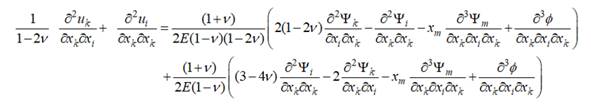
The Papkovich-Neuber procedure can be summarized as follows:

 

1. Begin by finding a vector function ${\Psi }_i(x_1,x_2,x_3)$ and scalar function $\varphi (x_1,x_2,x_3)$ which satisfy

${\displaystyle \frac{{\partial }^2{\Psi }_i}{\partial x_j\partial x_j}=-{\rho }_0{b}_i{\displaystyle \frac{{\partial }^2\varphi }{\partial x_k\partial x_k}=-{\rho }_0{b}_i{x}_i}}$

as well as boundary conditions

$\begin{array}{l}{\displaystyle \frac{2(1+\nu )}{E}\left({\Psi }_i+{\displaystyle \frac{1}{4(1-\nu )}{\displaystyle \frac{\partial }{\partial x_i}\left(\varphi -x_k{\Psi }_k\right)}}\right)=u_i^{*}\text{on }{\partial }_{1}R}\\ 2\nu {\displaystyle \frac{\partial {\Psi }_k}{\partial x_k}{n}_i+(1-2\nu )\left({\displaystyle \frac{\partial {\Psi }_i}{\partial x_j}+{\displaystyle \frac{\partial {\Psi }_j}{\partial x_i}}}\right)n_j-x_k{\displaystyle \frac{{\partial }^2{\Psi }_k}{\partial x_i\partial x_j}{n}_j+{\displaystyle \frac{{\partial }^2\varphi }{\partial x_i\partial x_j}{n}_j=2(1-\nu )t_i^{*}\text{on }{\partial }_{2}R}}}\end{array}$

 

2. Calculate displacements from the formula

$u_i={\displaystyle \frac{2(1+\nu )}{E}\left({\Psi }_i+{\displaystyle \frac{1}{4(1-\nu )}{\displaystyle \frac{\partial }{\partial x_i}\left(\varphi -x_k{\Psi }_k\right)}}\right)}$

 

3. Calculate stresses from the formula

$2(1-\nu ){\sigma }_{ij}=2\nu {\displaystyle \frac{\partial {\Psi }_k}{\partial x_k}{\delta }_{ij}+(1-2\nu )\left({\displaystyle \frac{\partial {\Psi }_i}{\partial x_j}+{\displaystyle \frac{\partial {\Psi }_j}{\partial x_i}}}\right)-x_k{\displaystyle \frac{{\partial }^2{\Psi }_k}{\partial x_i\partial x_j}+{\displaystyle \frac{{\partial }^2\varphi }{\partial x_i\partial x_j}}}}$

 

 

HEALTH WARNING: Although the displacements and stresses that solve a linear elasticity problem are unique, the Papkovich-Neuber potentials that generate a particular solution are not.   Consequently, if you find several different sets of potentials in the literature that claim to solve the same problem, don’t panic.   It is likely that they really do solve the same problem. 

 

 

 

5.4.2 Demonstration that the Papkovich-Neuber solution satisfies the governing equations

 

We need to show two things:

 

1. That the displacement field satisfies the equilibrium equation (See sect 5.1.2)

${\displaystyle \frac{1}{1-2\nu }{\displaystyle \frac{{\partial }^2{u}_k}{\partial x_k\partial x_i}+{\displaystyle \frac{{\partial }^2{u}_i}{\partial x_k\partial x_k}=-2(1+\nu ){\rho }_0{\displaystyle \frac{b_i}{E}}}}}$

 

2. That the stresses are related to the displacements by the elastic stress-strain equations

 

 

To show the first result, differentiate the formula relating potentials to the displacement to see that

${\displaystyle \frac{{\partial }^2{u}_k}{\partial x_i\partial x_j}={\displaystyle \frac{(1+\nu )}{2E(1-\nu )}\left((3-4\nu ){\displaystyle \frac{{\partial }^2{\Psi }_k}{\partial x_i\partial x_j}-{\displaystyle \frac{{\partial }^2{\Psi }_j}{\partial x_k\partial x_i}-{\displaystyle \frac{{\partial }^2{\Psi }_i}{\partial x_k\partial x_j}-x_m{\displaystyle \frac{{\partial }^3{\Psi }_m}{\partial x_k\partial x_i\partial x_j}+{\displaystyle \frac{{\partial }^3\varphi }{\partial x_k\partial x_i\partial x_j}}}}}}\right)}}$

Substitute this result into the governing equation to see that

Finally, substitute the governing equations for the potentials

${\displaystyle \frac{{\partial }^2{\Psi }_i}{\partial x_j\partial x_j}=-{\rho }_0{b}_i{\displaystyle \frac{{\partial }^2\varphi }{\partial x_k\partial x_k}=-{\rho }_0{b}_i{x}_i}}$

and simplify the result to verify that the governing equation is indeed satisfied. The second result can be derived by substituting the formula for displacement into the elastic stress-strain equations and simplifying.

 

 

 

5.4.3 Point force in an infinite solid

 

The displacements and stresses induced by a point force $P=P_1{e}_1+P_2{e}_2+P_3{e}_3$ acting at the origin of a large (infinite) elastic solid with Young’s modulus E and Poisson’s ratio $\nu$ are generated by the Papkovich-Neuber potentials

${\Psi }_i={\displaystyle \frac{P_i}{4\pi R}\varphi =0}$

where $R=\sqrt{x_i{x}_i}$. The displacements, strains and stresses follow as

$\begin{array}{l}{u}_i={\displaystyle \frac{(1+\nu )}{8\pi E(1-\nu )R}\left\{{\displaystyle \frac{P_k{x}_k{x}_i}{R^2}+(3-4\nu )P_i}\right\}}\\ {\epsilon }_{ij}={\displaystyle \frac{-(1+\nu )}{8\pi E(1-\nu )R^2}\left\{{\displaystyle \frac{3P_k{x}_k{x}_i{x}_j}{R^3}-{\displaystyle \frac{P_k{x}_k{\delta }_{ij}}{R}}}\right.+(1-2\nu )\left.{\displaystyle \frac{P_i{x}_j+P_j{x}_i}{R}}\right\}}\\ {\sigma }_{ij}^{}={\displaystyle \frac{-1}{8\pi (1-\nu )R^2}\left\{{\displaystyle \frac{3P_k{x}_k{x}_i{x}_j}{R^3}}\right.\left.+(1-2\nu ){\displaystyle \frac{P_i{x}_j+P_j{x}_i-{\delta }_{ij}{P}_k{x}_k}{R}}\right\}}\end{array}$

 

 

 

 

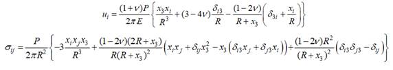
5.4.4 Point force normal to the surface of an infinite half-space

 

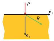The figure shows a point force $P=P{e}_3$ acting normal to the surface of a semi-infinite solid with Young’s modulus E and Poisson’s ratio $\nu$. The displacements and stresses in the half-space are generated by the Papkovich-Neuber potentials

${\Psi }_i={\displaystyle \frac{(1-\nu ){\delta }_{i3}}{\pi R}\varphi =-{\displaystyle \frac{(1-2\nu )(1-\nu )}{\pi }\log (R+x_3)}}$

where $R=\sqrt{x_k{x}_k}$

 

The displacements and stresses follow as

 

 

 

 

5.4.5 Point force tangent to the surface of an infinite half-space

 

The figure shows a point force $P=P{e}_1$ acting tangent to the surface of a semi-infinite solid with Young’s modulus E and Poisson’s ratio $\nu$. The stresses and displacements in the solids are generated by the Papkovich-Neuber potentials

$\begin{array}{l}{\Psi }_i={\displaystyle \frac{P}{2\pi (R+x_3)}\left({\delta }_{i1}-{\displaystyle \frac{x_2^2{\delta }_{i1}}{R(R+x_3)}+{\displaystyle \frac{x_1{x}_2{\delta }_{i2}}{R(R+x_3)}+2(1-\nu ){\displaystyle \frac{x_1{\delta }_{i3}}{R}}}}\right)}\\ \varphi ={\displaystyle \frac{P}{2\pi }\left(1+4{(1-\nu )}^2\right){\displaystyle \frac{x_1}{R+x_3}}}\end{array}$

The displacements and stresses can be calculated from these potentials as

$u_i={\displaystyle \frac{P(1+\nu )}{2\pi ER}\left\{{\delta }_{i1}+{\displaystyle \frac{x_1{x}_i}{R^2}+(1-2\nu )\left({\displaystyle \frac{R{\delta }_{i1}}{R+x_3}-{\displaystyle \frac{R{x}_1{\delta }_{i3}}{{(R+x_3)}^2}-{\displaystyle \frac{x_1{x}_i}{{(R+x_3)}^2}}}}\right)}\right\}}$

$\begin{array}{l}{\sigma }_{ij}={\displaystyle \frac{P}{2\pi }\left[-{\displaystyle \frac{3x_1{x}_i{x}_j}{R^5}+(1-2\nu )\left\{{\displaystyle \frac{x_1{x}_i{x}_j}{R^3{(R+x_3)}^2}+{\displaystyle \frac{2x_1{x}_i{x}_j}{R^2{(R+x_3)}^3}}}\right\}(1-{\delta }_{i3})(1-{\delta }_{j3})}\right.}\\ +(1-2\nu )\left.\left\{{\displaystyle \frac{x_1{x}_3(2R+x_3)}{R^3{(R+x_3)}^2}\left({\delta }_{i1}{\delta }_{j1}+{\delta }_{i2}{\delta }_{j2}\right)-{\displaystyle \frac{2x_1{\delta }_{i1}{\delta }_{j1}}{R{(R+x_3)}^2}-{\displaystyle \frac{x_2\left({\delta }_{i1}{\delta }_{j2}+{\delta }_{i2}{\delta }_{j1}\right)}{R{(R+x_3)}^2}}}}\right\}\right]\\ (\text{no sum on }i\text{ or }j)\end{array}$

 

 

 

5.4.6 The Eshelby Inclusion Problem

 

The Eshelby problem (Eshelby, 1957) is posed as follows:

 

1. Consider an infinite, isotropic, linear elastic solid, with (homogeneous) Young’s modulus and Poisson’s ratio $E,\nu$.

 

2. The solid is initially stress free, with displacements, strains and stresses $u_i={\epsilon }_{ij}={\sigma }_{ij}=0$.

 

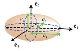
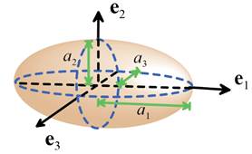
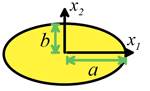
3. Some unspecified external agency then induces a uniform `transformation strain ${\epsilon }_{ij}^T$ inside an ellipsoidal region, with semi-axes $(a_1,a_2,a_3)$ centered at the origin (see the figure below) The ‘transformation strain’ can be visualized as an anisotropic thermal expansion $–$ if the ellipsoidal region were separated from the surrounding elastic solid, it would be stress free, and would change its shape according to the strain tensor ${\epsilon }_{ij}^T$.

 

 

4. Because the ellipsoid is encapsulated within the surrounding elastic solid, stress, strain and displacement fields are induced throughout the elastic solid.  These fields must be defined carefully because the initial configuration for the solid could be chosen in a number of different ways.  In the following, $u_i$ will denote the displacement of a material particle from the initial, unstressed configuration, as the transformation strain is introduced.   The total strain is defined as

${\epsilon }_{ij}=\left(\partial u_i/\partial x_j+\partial u_j/\partial x_i\right)/2$

Inside the ellipsoid, the total strain consists of the transformation strain  (which does not induce stress); together with an additional elastic strain ${\epsilon }_{ij}={\epsilon }_{ij}^T+{\epsilon }_{ij}^e$. Outside the ellipsoid, ${\epsilon }_{ij}={\epsilon }_{ij}^e$. The stress in the solid is related to the elastic part of the strain by the usual linear elastic equations

${\sigma }_{ij}={\displaystyle \frac{E}{1+\nu }\left\{{\epsilon }_{ij}^e+{\displaystyle \frac{\nu }{1-2\nu }{\epsilon }_{kk}^e{\delta }_{ij}}\right\}}$

 

The Eshelby solution gives full expressions for these fields.  It has proved to be one of the most important solutions in all of linear elasticity: it is of some interest in its own right, because it provides some insight into the mechanics of phase transformations in crystals.  More importantly, a number of very important boundary value problems can be solved by manipulating the Eshelby solution.  These include (i) the solution for an ellipsoidal inclusion embedded within an elastically mismatched matrix; (ii) the solution for an ellipsoidal cavity in an elastic solid; (iii) solutions for circular and elliptical cracks in an elastic solid.  In addition, the Eshelby solution is used extensively in theories that provide estimates of elastic properties of composite materials.

 

The displacement field is generated by Papkovich-Neuber potentials

${\Psi }_i(x_k)={\displaystyle \underset{S}{\int }{\displaystyle \frac{p_{ji}^T{n}_j(\xi )}{4\pi R(x,\xi )}}}dA(\xi )\varphi (x_k)={\displaystyle \underset{S}{\int }{\displaystyle \frac{{\xi }_i{p}_{ji}^T{n}_j(\xi )}{4\pi R(x,\xi )}}}dA(\xi )$

where the integral is taken over the surface of the ellipsoid, $n_j(\xi )$ denotes the components of a unit vector perpendicular to the surface of the ellipsoid (pointing outwards); $R=\sqrt{\left(x_k-{\xi }_k\right)\left(x_k-{\xi }_k\right)}$, and

$p_{ij}^T={\displaystyle \frac{E}{1+\nu }\left\{{\epsilon }_{ij}^T+{\displaystyle \frac{\nu }{1-2\nu }{\epsilon }_{kk}^T{\delta }_{ij}}\right\}}$

is the transformation stress (i.e. the stress that would be induced by applying an elastic strain to the inclusion that is equal to the transformation strain).  The stresses outside the inclusion can be calculated using the standard Papkovich-Neuber representation given in Section 5.4.1.  To calculate stresses inside the inclusion, the formula must be modified to account for the transformation strain, which gives

$2(1-\nu ){\sigma }_{ij}=-2(1-\nu )p_{ij}^T+2\nu {\displaystyle \frac{\partial {\Psi }_k}{\partial x_k}{\delta }_{ij}+(1-2\nu )\left({\displaystyle \frac{\partial {\Psi }_i}{\partial x_j}+{\displaystyle \frac{\partial {\Psi }_j}{\partial x_i}}}\right)-x_k{\displaystyle \frac{{\partial }^2{\Psi }_k}{\partial x_i\partial x_j}+{\displaystyle \frac{{\partial }^2\varphi }{\partial x_i\partial x_j}}}}$

For the general ellipsoid, the expressions for displacement and stress can be reduced to elliptic integrals, with the results

 

Solution inside the ellipsoid: Remarkably, it turns out that the stresses and strains are uniform inside the ellipsoid.  The displacements, strains and stresses can be expressed as:

 

(i) Displacement $u_i=\left(S_{ijkl}^{\ast }+{\Pi }_{ijkl}\right){\epsilon }_{kl}^T{x}_j$

 

(ii) Strain ${\epsilon }_{ij}={\epsilon }_{ij}^e+{\epsilon }_{ij}^T=S_{ijkl}^{\ast }{\epsilon }_{kl}^T$

 

(iii) Stress ${\sigma }_{ij}={\displaystyle \frac{E}{1+\nu }\left(S_{ijkl}^{*}{\epsilon }_{kl}^T+{\displaystyle \frac{\nu }{1-2\nu }{\delta }_{ij}{S}_{ppkl}^{*}{\epsilon }_{kl}^T}\right)-p_{ij}^T}$

 

 

Here, $S_{ijkl}^{*}$ is a constant called the `Eshelby Tensor,’ and ${\Pi }_{ijkl}$ is a second (anonymous) constant tensor. These tensors can be calculated as follows. Choose the coordinate system so that $a_1>a_2>a_3$. Define

$\begin{array}{l}{I}_1={\displaystyle \frac{4\pi a_1{a}_2{a}_3}{(a_1^2-a_2^2)\sqrt{(a_1^2-a_3^2)}}\left(F(\theta ,k)-E(\theta ,k)\right)}\\ I_3={\displaystyle \frac{4\pi a_1{a}_2{a}_3}{(a_2^2-a_3^2)\sqrt{(a_1^2-a_3^2)}}\left\{{\displaystyle \frac{a_2{(a_1^2-a_3^2)}^{1/2}}{a_1{a}_3}-E(\theta ,k)}\right\}}\\ I_2=4\pi -I_1-I_3\\ I_{ij}=(I_j-I_i)/\left[3(a_i^2-a_j^2)\right](i\ne j,\text{no sum on }i,j)\\ I_{11}=4\pi /\left(3a_1^2\right)-I_{12}-I_{13}\\ I_{22}=4\pi /\left(3a_2^2\right)-I_{23}-I_{21}\\ I_{33}=4\pi /\left(3a_3^2\right)-I_{31}-I_{32}\end{array}$

where $\theta ={\sin }^{-1}\sqrt{(1-a_3^2/a_1^2)}{k}^2=(a_1^2-a_2^2)/(a_1^2-a_3^2)$ and

$F(\theta ,k)={\displaystyle \underset{0}{\overset{\theta }{\int }}{\displaystyle \frac{dw}{{(1-k^2{\sin }^{2}w)}^{1/2}}}}E(\theta ,k)={\displaystyle \underset{0}{\overset{\theta }{\int }}{(1-k^2{\sin }^{2}w)}^{1/2}dw}$

are elliptic integrals of the first and second kinds.  Then

$\begin{array}{l}{S}^{\ast }{}_{1111}={\displaystyle \frac{3}{8\pi (1-\nu )}{a}_1^2{I}_{11}+{\displaystyle \frac{1-2\nu }{8\pi (1-\nu )}{I}_1}}\\ S^{\ast }{}_{1122}={\displaystyle \frac{3}{8\pi (1-\nu )}{a}_2^2{I}_{12}-{\displaystyle \frac{1-2\nu }{8\pi (1-\nu )}{I}_1}}\\ S^{\ast }{}_{1133}={\displaystyle \frac{3}{8\pi (1-\nu )}{a}_3^2{I}_{13}-{\displaystyle \frac{1-2\nu }{8\pi (1-\nu )}{I}_1}}\\ S^{\ast }{}_{1212}={\displaystyle \frac{a_1^2+a_2^2}{16\pi (1-\nu )}{I}_{12}+{\displaystyle \frac{1-2\nu }{16\pi (1-\nu )}(I_1+I_2)}}\\ {\Pi }_{ijij}=(I_i-I_j)/8\pi i\ne j\end{array}$

The remaining components of $S_{ijkl}^{*}$ can be calculated by cyclic permutations of (1,2,3).  Any components that cannot be obtained from these formulas are zero: thus $S_{1112}^{\ast }=S_{1223}^{\ast }=S_{1232}^{\ast }=0$, ${\Pi }_{1112}=0$, etc.  Note that $S_{ijkl}^{*}$ has many of the symmetries of the elastic compliance tensor (e.g $S_{ijkl}^{*}=S_{jikl}^{*}$ ), but does not have major symmetry $S_{ijkl}^{*}\ne S_{klij}^{*}$. 

 

 

For certain special shapes the expressions given for $I_k$ break down and simplified formulas must be used

 

Oblate spheroid $a_1=a_2>a_3$ 

$\begin{array}{l}{I}_1=I_2={\displaystyle \frac{2\pi a_1{a}_2{a}_3}{{\left(a_1^2-a_3^2\right)}^{3/2}}\left\{{\cos }^{-1}{\displaystyle \frac{a_3}{a_1}-{\displaystyle \frac{a_3}{a_1}{\left(1-{\displaystyle \frac{a_3^2}{a_1^2}}\right)}^{1/2}}}\right\}}\\ I_{12}=I_{21}=\pi /\left(3a_1^2\right)-I_{13}/4\end{array}$

 

Prolate spheroid $a_1>a_2=a_3$

$\begin{array}{l}{I}_2=I_3={\displaystyle \frac{2\pi a_1{a}_2{a}_3}{{\left(a_1^2-a_3^2\right)}^{3/2}}\left\{{\displaystyle \frac{a_1}{a_3}{\left({\displaystyle \frac{a_1^2}{a_3^2}-1}\right)}^{1/2}-{\cosh }^{-1}{\displaystyle \frac{a_1}{a_3}}}\right\}}\\ I_{13}=I_{31}=\pi /3a_1^2-I_{12}/4\end{array}$

 

Sphere $a_1=a_2=a_3$. In this case the Eshelby tensor can be calculated analytically

$\begin{array}{l}{S}_{1111}^{\ast }=S_{2222}^{\ast }=S_{3333}^{\ast }={\displaystyle \frac{7-5\nu }{15(1-\nu )}}\\ S_{1212}^{\ast }=S_{2323}^{\ast }=S_{3131}^{\ast }={\displaystyle \frac{4-5\nu }{15(1-\nu )}}\\ S_{1122}^{\ast }=S_{2233}^{\ast }=S_{3311}^{\ast }=S_{1133}^{\ast }=S_{2211}^{\ast }=S_{3322}^{\ast }={\displaystyle \frac{5\nu -1}{15(1-\nu )}}\\ \end{array}$

Additional terms follow from the symmetry conditions $S_{ijkl}=S_{jikl}=S_{ijlk}=S_{jilk}$.  The remaining terms are zero.

 

Cylinder $a_3\to \infty$. For this case the Eshelby tensor reduces to

$\begin{array}{l}{S}_{1111}^{*}={\displaystyle \frac{a_2\left[2(1-\nu )(a_1+a_2)+a_1\right]}{2(1-\nu ){(a_1+a_2)}^2}{S}_{2222}^{*}={\displaystyle \frac{a_1\left[2(1-\nu )(a_1+a_2)+a_2\right]}{2(1-\nu ){(a_1+a_2)}^2}{S}_{3333}^{*}=0}}\\ S_{1122}^{*}={\displaystyle \frac{a_2\left[(2\nu -1)a_1+2\nu a_2\right]}{2(1-\nu ){(a_1+a_2)}^2}{S}_{2211}^{*}={\displaystyle \frac{a_1\left[(2\nu -1)a_2+2\nu a_1\right]}{2(1-\nu ){(a_1+a_2)}^2}}}\\ S_{1133}^{*}={\displaystyle \frac{\nu a_2}{(1-\nu )(a_1+a_2)}{S}_{3311}^{*}=0}\\ S_{2233}^{*}={\displaystyle \frac{\nu a_1}{(1-\nu )(a_1+a_2)}{S}_{3322}^{*}=0S_{1212}^{*}={\displaystyle \frac{\left[(1-\nu )(a_1^2+a_2^2)+(1-2\nu )a_1{a}_2\right]}{2(1-\nu ){(a_1+a_2)}^2}}}\\ S_{1313}^{*}={\displaystyle \frac{a_2(2-\nu )}{2(1-\nu )(a_1+a_2)}{S}_{2323}^{*}={\displaystyle \frac{a_1(2-\nu )}{2(1-\nu )(a_1+a_2)}}}\end{array}$

Additional terms follow from the symmetry conditions $S_{ijkl}=S_{jikl}=S_{ijlk}=S_{jilk}$.  The remaining terms are zero.

 

Solution outside the ellipsoid: The solution outside the ellipsoid can also be expressed in simplified form: Eshelby (1959) shows that the displacement can be obtained from a single scalar potential $\omega (x_i)$.  For actual calculations only the derivatives of the potential are required, which can be reduced to

$\begin{array}{l}{\displaystyle \frac{d\omega }{d{x}_1}={\displaystyle \frac{x_1{a}_1{a}_2{a}_3}{l^3{k}^2}\left\{E(\theta ,k)-F(\theta ,k)\right\}}}\\ {\displaystyle \frac{d\omega }{d{x}_2}={\displaystyle \frac{x_2{a}_1{a}_2{a}_3}{l^3{k}^2{\widehat{k}}^2}\left\{{\widehat{k}}^{2}F(\theta ,k)-E(\theta ,k)+l{A}_3{k}^2/(A_1{A}_2)\right\}}}\\ {\displaystyle \frac{d\omega }{d{x}_3}={\displaystyle \frac{x_3{a}_1{a}_2{a}_3}{l^3{\widehat{k}}^2}\left\{E(\theta ,k)-l{A}_2/(A_1{A}_3)\right\}}}\end{array}$

$\begin{array}{l}{A}_i=\sqrt{a_i^2+\lambda }l=\sqrt{a_1^2-a_3^2}\\ k=\sqrt{(a_1^2-a_2^2)/(a_1^2-a_3^2)}\widehat{k}=\sqrt{(a_2^2-a_3^2)/(a_1^2-a_3^2)}\end{array}$

where $\lambda$ is the greatest positive root of ${\lambda }^3-L{\lambda }^2+M\lambda -N=0$, with

$L=r^2-R^{2}M={\displaystyle \sum _{i=1}^3{a}_i^2{x}_i}-a_1^2{a}_2^2-a_2^2{a}_3^2-a_1^2{a}_3^2+r^2{R}^{2}N=a_1^2{a}_2^2{a}_3^2\left({\displaystyle \sum _{i=1}^3{\displaystyle \frac{x_i^2}{a_i^2}-1}}\right)$

and $r=\sqrt{x_k{x}_k}R=\sqrt{a_k{a}_k}$.  Additional derivatives can be computed using the relations

$dF/d\lambda =-l/(2A_1{A}_2{A}_3)dE/d\lambda =-l{A}_2/(A_1^3{A}_3)d\lambda /d{x}_i=2x_i/(A_{i}h)h^2={\displaystyle \sum _{i=1}^3{x}_i^2/A_i^4}$

The displacements follow as

$\begin{array}{l}2(1-\nu )u_1={\displaystyle \frac{{\epsilon }_{11}^T-{\epsilon }_{22}^T}{a_1^2-a_2^2}{\displaystyle \frac{\partial }{\partial x_2}\left(a_1^2{x}_2{\displaystyle \frac{\partial \omega }{\partial x_1}-a_2^2{x}_1{\displaystyle \frac{\partial \omega }{\partial x_2}}}\right)+{\displaystyle \frac{{\epsilon }_{33}^T-{\epsilon }_{11}^T}{a_3^2-a_1^2}{\displaystyle \frac{\partial }{\partial x_3}\left(a_3^2{x}_1{\displaystyle \frac{\partial \omega }{\partial x_3}-a_1^2{x}_3{\displaystyle \frac{\partial \omega }{\partial x_3}}}\right)}}}}\\ -2\left\{(1-\nu ){\epsilon }_{11}^T+\nu ({\epsilon }_{11}^T+{\epsilon }_{22}^T)\right\}{\displaystyle \frac{\partial \omega }{\partial x_1}-4(1-\nu )\left({\epsilon }_{12}^T{\displaystyle \frac{\partial \omega }{\partial x_2}+{\epsilon }_{13}^T{\displaystyle \frac{\partial \omega }{\partial x_3}}}\right)+{\displaystyle \frac{\partial \beta }{\partial x_1}}}\end{array}$

where

$\begin{array}{l}\beta ={\displaystyle \frac{2{\epsilon }_{12}^T}{a_1^2-a_2^2}\left(a_1^2{x}_2{\displaystyle \frac{\partial \omega }{\partial x_1}-a_2^2{x}_1{\displaystyle \frac{\partial \omega }{\partial x_2}}}\right)+{\displaystyle \frac{2{\epsilon }_{23}^T}{a_2^2-a_3^2}\left(a_2^2{x}_3{\displaystyle \frac{\partial \omega }{\partial x_2}-a_3^2{x}_2{\displaystyle \frac{\partial \omega }{\partial x_3}}}\right)}}\\ +{\displaystyle \frac{2{\epsilon }_{31}^T}{a_3^2-a_1^2}\left(a_3^2{x}_1{\displaystyle \frac{\partial \omega }{\partial x_3}-a_1^2{x}_3{\displaystyle \frac{\partial \omega }{\partial x_1}}}\right)}\end{array}$

The remaining displacement components can be calculated by cyclic permutations of (1,2,3), and strains and stresses can be calculated by differentiating the displacements appropriately.  The results are far too complicated to write out in full, and in practice the algebra can only be done with the aid of a symbolic manipulation program.  Some special results can be reduced to a tractable form, however:

 

Displacements far from the ellipsoid $R=\sqrt{x_k{x}_k}>>a_1$

$u_i={\displaystyle \frac{a_1{a}_2{a}_3}{8(1-\nu )R^2}\left\{{\displaystyle \frac{3{\epsilon }_{jk}^T{x}_i{x}_j{x}_k}{R^3}+(1-2\nu ){\displaystyle \frac{2{\epsilon }_{ik}^T{x}_k-{\epsilon }_{kk}^T{x}_i}{R}}}\right\}}$

 

Solution outside a spherical inclusion: For this case the Papkovich-Neuber potentials can be reduced to

${\Psi }_i={\displaystyle \frac{a^3{p}_{ik}^T{x}_k}{3R^3}\varphi ={\displaystyle \frac{a^3{p}_{ij}^T}{15R^3}\left((5R^2-a^2){\delta }_{ij}+3a^2{\displaystyle \frac{x_i{x}_j}{R^2}}\right)}}$

The displacements and stresses follow as

$u_i={\displaystyle \frac{(1+\nu )a^3}{2(1-\nu )E}\left\{{\displaystyle \frac{(2p_{ik}^T{x}_k+p_{kk}^T{x}_i)}{15R^5}(3a^2-5R^2)+{\displaystyle \frac{p_{jk}^T{x}_j{x}_k{x}_i}{R^7}(R^2-a^2)+{\displaystyle \frac{4(1-\nu )p_{ik}^T{x}_k}{3R^3}}}}\right\}}$

$\begin{array}{l}{\sigma }_{ij}={\displaystyle \frac{a^3}{2(1-\nu )R^3}\left\{{\displaystyle \frac{p_{ij}^T}{15}\left(10(1-2\nu )+6{\displaystyle \frac{a^2}{R^2}}\right)}\right.+{\displaystyle \frac{p_{ik}^T{x}_k{x}_j+p_{jk}^T{x}_k{x}_i}{R^2}\left(2\nu -2{\displaystyle \frac{a^2}{R^2}}\right)}}\\ +{\displaystyle \frac{{\delta }_{ij}{p}_{kk}^T}{15}\left(3{\displaystyle \frac{a^2}{R^2}-5(1-2\nu )}\right)+{\displaystyle \frac{{\delta }_{ij}{p}_{kl}^T{x}_k{x}_l}{R^2}\left((1-2\nu )-{\displaystyle \frac{a^2}{R^2}}\right)}}\\ -\left.{\displaystyle \frac{x_i{x}_j{p}_{kl}^T{x}_k{x}_l}{R^4}\left(5-7{\displaystyle \frac{a^2}{R^2}}\right)+{\displaystyle \frac{x_i{x}_j{p}_{kk}^T}{R^2}\left(1-{\displaystyle \frac{a^2}{R^2}}\right)}}\right\}\end{array}$

where $R=\sqrt{x_k{x}_k}$ and $p_{ij}^T=\left\{E/(1+\nu )\right\}\left\{{\epsilon }_{ij}^T+\nu {\epsilon }_{kk}^T{\delta }_{ij}/(1-2\nu )\right\}$

 

 

 

5.4.7 Elastically mismatched ellipsoidal inclusion in an infinite solid subjected to remote stress

 

The figure below shows an ellipsoidal inclusion, with semi-axes $(a_1,a_2,a_3)$.  The inclusion is made from an isotropic, elastic solid with Young’s modulus $E^I$ and Poisson’s ratio ${\nu }^I$.  It is embedded in an infinite, isotropic elastic matrix with Young’s modulus $E^M$ and Poisson’s ratio ${\nu }^M$.  The solid is loaded at infinity by a uniform stress state ${\sigma }_{ij}^{\infty }$, strains ${\epsilon }_{ij}^{\infty }=((1+{\nu }^M){\sigma }_{ij}^{\infty }-{\nu }^M{\sigma }_{kk}^{\infty }{\delta }_{ij})/E^M$ and displacements $u_i^{\infty }={\epsilon }_{ij}^{\infty }{x}_j$.

 

 

The solution is constructed by superposing the Eshelby solution to the uniform stress state.  To represent the Eshelby solution, we introduce:

 

1. The Eshelby transformation strain ${\epsilon }_{ij}^T$

 

2. The Eshelby tensor $S_{ijkl}^{*}$

 

3. The displacement induced by the Eshelby transformation $u_i=U_{ikl}(x_m){\epsilon }_{kl}^T$

 

4. The stresses induced by the Eshelby transformation ${\sigma }_{ij}={\Sigma }_{ijkl}(x_m){\epsilon }_{kl}^T$

 

 

The functions $S_{ijkl}^{*}$ $U_{ikl}$ and ${\Sigma }_{ijkl}$ can be calculated using the results given in Section 5.4.6 (the elastic properties of the matrix should be used when evaluating the formulas).

 

The solution for the solid containing the inclusion follows as

$u_i=U_{ikl}(x_m){\epsilon }_{kl}^T+u_i^{\infty }{\sigma }_{ij}={\Sigma }_{ijkl}(x_m){\epsilon }_{kl}^T+{\sigma }_{ij}^{\infty }$

where the transformation strain is calculated by solving

$(C_{ijkl}^M-C_{ijkl}^I){\epsilon }_k^{\infty }{,}_l=(C_{ijpq}^M-(C_{ijkl}^M-C_{ijkl}^I)S_{klpq}^{\ast }){\epsilon }_{pq}^T$

for ${\epsilon }_{ij}^T$.  Here,

$C_{ijkl}^M={\displaystyle \frac{E^M}{2\left(1+{\nu }^M\right)}\left({\delta }_{il}{\delta }_{jk}+{\delta }_{ik}{\delta }_{jl}\right)+{\displaystyle \frac{E^M{\nu }^M}{\left(1+{\nu }^M\right)\left(1-2{\nu }^M\right)}{\delta }_{ij}{\delta }_{kl}}}$

is the stiffness of the matrix, with a similar expression for the stiffness of the inclusion.

 

 

 

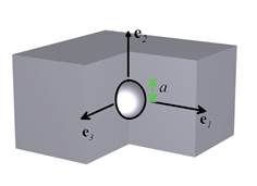
5.4.8 Spherical cavity in an infinite solid subjected to remote stress

 

The figure below shows a spherical cavity with radius a in an infinite, isotropic linear elastic solid. Far from the cavity, the solid is subjected to a tensile stress ${\sigma }_{33}={\sigma }_0$, with all other stress components zero.

 

The solution is generated by potentials

$\begin{array}{l}{\Psi }_i={\displaystyle \frac{(1-\nu ){\sigma }_0}{(1+\nu )}{x}_3{\delta }_{i3}+{\displaystyle \frac{a^3(1-\nu ){\sigma }_0}{R^3(7-5\nu )}\left({\displaystyle \frac{(5\nu -1)}{2(1-2\nu )}{x}_i+5x_3{\delta }_{i3}}\right)}}\\ \varphi ={\displaystyle \frac{\nu (1-\nu ){\sigma }_0}{(1+\nu )}(3x_3^2-R^2)+{\displaystyle \frac{a^3(1-\nu ){\sigma }_0}{R^3(7-5\nu )}\left({\displaystyle \frac{(7-5\nu )}{2(1-2\nu )}{R}^2-a^2+{\displaystyle \frac{3x_3^2{a}^2}{R^2}}}\right)}}\end{array}$

The displacements and stresses follow as

$\begin{array}{l}{u}_i={\displaystyle \frac{(1+\nu ){\sigma }_0}{E}\left\{1+{\displaystyle \frac{5}{7-5\nu }\left(1-2\nu +{\displaystyle \frac{3}{5}{\displaystyle \frac{a^2}{R^2}}}\right){\displaystyle \frac{a^3}{R^3}}}\right\}{\delta }_{i3}{x}_3}\\ +{\displaystyle \frac{(1+\nu ){\sigma }_0}{E}\left(-{\displaystyle \frac{\nu }{(1+\nu )}-{\displaystyle \frac{6-5\nu }{7-5\nu }{\displaystyle \frac{a^3}{R^3}+{\displaystyle \frac{15}{2(7-5\nu )}{\displaystyle \frac{a^3}{R^3}\left({\displaystyle \frac{a^2}{5R^2}+{\displaystyle \frac{x_3^2}{R^2}-{\displaystyle \frac{a^2{x}_3^2}{R^4}}}}\right)}}}}}\right)x_i}\end{array}$

 

$\begin{array}{l}{\displaystyle \frac{{\sigma }_{ij}}{{\sigma }_0}={\delta }_{i3}{\delta }_{j3}\left\{1+{\displaystyle \frac{5(1-2\nu )}{(7-5\nu )}{\displaystyle \frac{a^3}{R^3}+{\displaystyle \frac{3}{(7-5\nu )}{\displaystyle \frac{a^5}{R^5}}}}}\right\}}\\ +{\displaystyle \frac{3}{2(7-5\nu )}{\displaystyle \frac{a^3}{R^3}{\delta }_{ij}\left\{(5\nu -2)+5(1-2\nu ){\displaystyle \frac{x_3^2}{R^2}+{\displaystyle \frac{a^2}{R^2}-5{\displaystyle \frac{a^2{x}_3^2}{R^4}}}}\right\}}}\\ +{\displaystyle \frac{3}{2(7-5\nu )}{\displaystyle \frac{a^3{x}_i{x}_j}{R^5}\left\{(6-5\nu )-25{\displaystyle \frac{x_3^2}{R^2}-5{\displaystyle \frac{a^2}{R^2}+35{\displaystyle \frac{x_3^2{a}^2}{R^4}}}}\right\}}}\\ -{\displaystyle \frac{15(1-\nu )}{7-5\nu }{\displaystyle \frac{({\delta }_{i3}{x}_j+{\delta }_{j3}{x}_i)a^3{x}_3}{R^5}}}\end{array}$

 

 

Derivation: This solution can be derived by superposing two solutions:

 

1. A uniform state of stress ${\sigma }_{ij}={\sigma }_0{\delta }_{i3}{\delta }_{j3}$, which can be generated from potentials

${\Psi }_i=(1-\nu ){\sigma }_0{x}_3{\delta }_{i3}/(1+\nu )\varphi =\nu (1-\nu ){\sigma }_0(3x_3^2-R^2)/(1+\nu )$,

 

2. The Eshelby solution for a sphere with transformation stress $p_{ij}^T=A{\delta }_{ij}+B{\delta }_{i3}{\delta }_{j3}$.

 

 

 The unknown coefficients A and B must be chosen to satisfy the traction free boundary condition ${\sigma }_{ij}{n}_j=0$ on the surface of the hole $R=a$.  Noting that $n_j=-x_j/a$ and working through some tedious algebra shows that

$A={\displaystyle \frac{3{\sigma }_0(1-\nu )(5\nu -1)}{2(7-5\nu )(1-2\nu )}B={\displaystyle \frac{15{\sigma }_0(1-\nu )}{(7-5\nu )}}}$

Substituting back into the Eshelby potentials and simplifying yields the results given.  The same approach can be used to derive the solution for a rigid inclusion in an infinite solid subjected to remote stress, as well as the solution to an elastically mismatched spherical inclusion in an infinite solid.

 

 

 

5.4.9 Flat ended cylindrical indenter in contact with an elastic half-space

 

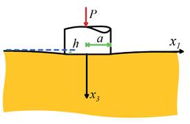The figure shows a rigid, flat ended, cylindrical punch with radius a, which is pushed into the surface of an elastic half-space with Young’s modulus E and Poisson’s ratio $\nu$ by a force P.  The indenter sinks into the surface by a depth h. The interface between the contacting surfaces is frictionless

 

The load is related to the displacement of the punch by

$P={\displaystyle \frac{2Ea}{(1-{\nu }^2)}h}$

 

The solution can be generated from Papkovich-Neuber potentials

$\begin{array}{l}{\Psi }_k={\displaystyle \frac{2Eh{\delta }_{k3}}{(1+\nu )\pi }\mathrm{Im}\left\{\log \left(R^{*}+x_3+ia\right)\right\}}\\ \varphi =-{\displaystyle \frac{2(1-2\nu )Eh}{(1+\nu )\pi }\mathrm{Im}\left\{(x_3+ia)\log \left(R^{*}+x_3+ia\right)-R^{*}\right\}}\end{array}$

where $R^{*}=\sqrt{x_1^2+x_2^2+{(x_3+ia)}^2}$, $i=\sqrt{-1}$ and $\mathrm{Im}\left\{z\right\}$ denotes the imaginary part of z.  The displacements and stresses follow as

$u_k={\displaystyle \frac{h}{\pi (1-\nu )}\mathrm{Im}\left\{2(1-\nu ){\delta }_{k3}\log \left(R^{*}+x_3+ia\right)-{\displaystyle \frac{x_3{\delta }_{k3}}{R^{*}}+{\displaystyle \frac{x_1{\delta }_{k1}+x_2{\delta }_{k2}}{R^{*}+x_3+ia}\left(1-2\nu -{\displaystyle \frac{x_3}{R^{*}}}\right)}}\right\}}$

$\begin{array}{l}{\sigma }_{11}={\displaystyle \frac{Eh}{(1-{\nu }^2)\pi }\mathrm{Im}\left\{{\displaystyle \frac{2\nu }{R^{*}}+{\displaystyle \frac{1-2\nu -x_3/R^{*}}{R^{*}+x_3+ia}-{\displaystyle \frac{x_1^2}{R^{*}{(R^{*}+x_3+ia)}^2}\left(1+{\displaystyle \frac{x_3(1+2R^{*}+x_3+ia)}{R^{*2}}}\right)}}}\right\}}\\ {\sigma }_{22}={\displaystyle \frac{Eh}{(1-{\nu }^2)\pi }\mathrm{Im}\left\{{\displaystyle \frac{2\nu }{R^{*}}+{\displaystyle \frac{1-2\nu -x_3/R^{*}}{R^{*}+x_3+ia}-{\displaystyle \frac{x_2^2}{R^{*}{(R^{*}+x_3+ia)}^2}\left(1+{\displaystyle \frac{x_3(1+2R^{*}+x_3+ia)}{R^{*2}}}\right)}}}\right\}}\\ {\sigma }_{33}={\displaystyle \frac{Eh}{(1-{\nu }^2)\pi }\mathrm{Im}\left\{{\displaystyle \frac{1}{R^{*}}+{\displaystyle \frac{(x_3+ia)x_3}{R^{*3}}}}\right\}}\\ {\sigma }_{13}={\displaystyle \frac{Eh}{(1-{\nu }^2)\pi }\mathrm{Im}\left\{{\displaystyle \frac{x_1{x}_3}{R^{*3}}}\right\}}\\ {\sigma }_{23}={\displaystyle \frac{Eh}{(1-{\nu }^2)\pi }\mathrm{Im}\left\{{\displaystyle \frac{x_2{x}_3}{R^{*3}}}\right\}}\\ {\sigma }_{12}={\displaystyle \frac{Eh}{(1-{\nu }^2)\pi }\mathrm{Im}\left\{{\displaystyle \frac{x_1{x}_2}{R^{*}(R^{*}+x_3+ia)}\left(-(1-2\nu )+{\displaystyle \frac{x_3(2R^{*}+x_3+ia)}{R^{*}(R^{*}+x_3+ia)}}\right)}\right\}}\end{array}$

A symbolic manipulation program can handle the complex arithmetic in these formulas without difficulty. 

 

Important features of these results include:

 

1. Contact pressure: The pressure exerted by the indenter on the elastic solid follows as

$p(x_1)=-{\sigma }_{33}(r,x_3=0)={\displaystyle \frac{P}{2\pi a\sqrt{a^2-r^2}}}$

 

2. Surface displacement: The vertical displacement of the surface is

$u_3=\left\{\begin{array}{c}{\displaystyle \frac{2h}{\pi }{\tan }^{-1}{\displaystyle \frac{a}{\sqrt{r^2-a^2}}r>a}}\\ hr<a\end{array}\right.$

 

3. Contact stiffness: the stiffness of a contact is defined as the ratio of the force acting on the indenter to its displacement $k_c=P/h$, and is of interest in practical applications.  The stiffness of a 3D contact is well defined (unlike 2D contacts discussed in Section 5.4) and is given by $k_c=2Ea/(1-{\nu }^2)$.  This turns out to be a universal relation for any axisymmetric contact with contact radius a.

 

 

 

5.4.10 Frictionless contact between two elastic spheres

 

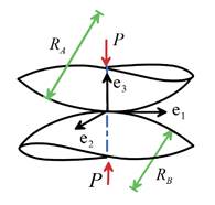This solution is known as the `Hertz contact problem’ after its author.  The figure illustrates the problem to be solved.  Two elastic spheres, with radii $R_A,R_B$ and elastic constants $E_A,{\nu }_A$, $E_B,{\nu }_B$ initially meet at a point, and are pushed into contact by a force P.  The two spheres deform so as to make contact over a small circular patch with radius $a<<R_B,R_B$, and the centers of the two spheres approach one another by a distance h.

 

 

The solution is conveniently expressed in terms of an effective modulus and radius for the contact pair:

$E^{*}={\displaystyle \frac{E_A{E}_B}{(1-{\nu }_A^2)E_B+(1-{\nu }_B^2)E_A}{R}^{*}={\displaystyle \frac{R_A{R}_B}{R_A+R_B}}}$

 

Relations between $P,h,a$:  The force P, approach of distant points h and contact area a are related by

$a={\left({\displaystyle \frac{3P{R}^{*}}{4E^{*}}}\right)}^{1/3}h={\displaystyle \frac{a^2}{R^{*}}={\left({\displaystyle \frac{9P^2}{16R^{*}{E}^{*2}}}\right)}^{1/3}}$

 

Contact pressure:  The two solids are subjected to a repulsive pressure $p(r)=p_0\sqrt{1-r^2/a^2}$ within the contact area.  The maximum contact pressure is related to the load applied to the spheres by

$p_0=\left({\displaystyle \frac{3P}{2\pi a^2}}\right)={\left({\displaystyle \frac{6P{E}^{*2}}{{\pi }^3{R}^{*2}}}\right)}^{1/3}$

 

Contact stiffness: the stiffness of a contact is defined as the ratio of the force acting on the indenter to its displacement $k_c=dP/dh$, and is of interest in practical applications.  The stiffness of a 3D contact is well defined (unlike 2D contacts discussed in Section 5.4) and is given by  $k_c=2E^{*}a$.  This turns out to be a universal relation for any axisymmetric contact with contact radius a.

 

Stress field: The two spheres are subjected to the same contact pressure, and are both assumed to deform like a half-space (with a flat surface).  Consequently, the stress field is identical inside both spheres, and can be calculated from formulas derived by Hamilton, (1983)

$\begin{array}{l}{\sigma }_{11}={\displaystyle \frac{p_0}{a}\left[\varphi +{\displaystyle \frac{x_2^2-x_1^2}{r^4}\left((1-\nu )N{x}_3^2-{\displaystyle \frac{1-2\nu }{3}\left(NS+2AN+a^3\right)-\nu M{x}_{3}a}\right)}\right.}\\ \left.-N{\displaystyle \frac{(x_1^2+2\nu x_2^2)}{r^2}-{\displaystyle \frac{M{x}_1^2{x}_{3}a}{S{r}^2}}}\right]\\ {\sigma }_{22}={\displaystyle \frac{p_0}{a}\left[\varphi +{\displaystyle \frac{x_1^2-x_2^2}{r^4}\left((1-\nu )N{x}_3^2-{\displaystyle \frac{1-2\nu }{3}\left(NS+2AN+a^3\right)-\nu M{x}_{3}a}\right)}\right.}\\ \left.-N{\displaystyle \frac{(x_2^2+2\nu x_1^2)}{r^2}-{\displaystyle \frac{M{x}_2^2{x}_{3}a}{S{r}^2}}}\right]\\ {\sigma }_{33}={\displaystyle \frac{p_0}{a}\left(-N+{\displaystyle \frac{a{x}_{3}M}{S}}\right){\sigma }_{13}=-{\displaystyle \frac{x_3{x}_1{p}_0}{a}\left({\displaystyle \frac{N}{S}-{\displaystyle \frac{x_{3}H}{G^2+H^2}}}\right)}}\\ {\sigma }_{23}=-{\displaystyle \frac{x_3{x}_2{p}_0}{a}\left({\displaystyle \frac{N}{S}-{\displaystyle \frac{x_{3}H}{G^2+H^2}}}\right)}\\ {\sigma }_{12}={\displaystyle \frac{p_0{x}_1{x}_2}{a{r}^4}\left[(1-2\nu )\left\{-N{r}^2+{\displaystyle \frac{2}{3}N(S+2A)-x_3(x_{3}N+aM)+{\displaystyle \frac{2}{3}{a}^3}}\right\}\right.}\\ \left.+x_3\left\{-{\displaystyle \frac{aM{r}^2}{S}-x_{3}N+aM}\right\}\right]\end{array}$

where

$\begin{array}{l}r=\sqrt{x_1^2+x_2^2}A=r^2+x_3^2-a^2\\ S=\sqrt{A^2+4a^2{x}_3^2}M=\sqrt{(S+A)/2}N=\sqrt{(S-A)/2}\\ G=M^2-N^2+x_{3}M-aNH=2MN+aM+x_{3}N\\ \varphi =(1+\nu )x_3{\tan }^{-1}(a/M)\end{array}$

The stresses on r=0 must be computed using a limiting process, with the result

${\sigma }_{11}={\sigma }_{22}={\displaystyle \frac{p_0}{a}\left[\left(1+\nu \right)\left(x_3{\tan }^{-1}(a/x_3)-a\right)+{\displaystyle \frac{a^3}{2\left(a^2+x_3^2\right)}}\right]{\sigma }_{33}=-{\displaystyle \frac{p_0{a}^2}{a^2+x_3^2}}}$

 

Conditions to initiate yield: The material under the contact yields when the maximum von-Mises effective stress ${\sigma }_e=\sqrt{3S_{ij}{S}_{ij}/2}$ reaches the uniaxial tensile yield stress Y.  The location of the maximum von-Mises stress can be found by plotting contours of ${\sigma }_e/p_0$ as a function of $x_1/a,x_3/a$.  For $\nu =0.3$ the maximum value occurs at $x_1=x_2=0,x_3=0.481a$ and has value ${\sigma }_e/p_0=0.6200$.  Yield occurs when $p_0=1.61Y$.

 

 

5.4.11 Contact area, pressure, stiffness and elastic limit for general non-conformal contacts

 

A non-conformal contact has the following properties: (i) the two contacting solids initially touch at a point or along a line; (ii) both contacting solids are smooth in the neighborhood of the contact, so that their local geometry can be approximated as ellipsoids, (iii) the size of the contact patch between the two solids is much smaller than either solid.

 

Complete solutions for such contacts can be found in Bryant and Keer (1982) or Sackfield and Hills (1983).  These papers also account for the effects of friction under sliding contacts.   The results are lengthy.  Here, we give formulas that predict the most important features of frictionless nonconformal contacts.

 

 

Contact Geometry: The geometry of the contacting solids is illustrated below.

 

 

The geometry is characterized as follows:

 

1. The principal radii of curvature of the two solids at the point of initial contact are denoted by ${\rho }_1^A,{\rho }_2^A$, ${\rho }_1^B,{\rho }_2^B$.  The radii of curvature are positive if convex and negative if concave. 

 

2. The angle between the principal directions of curvature of the two solids is denoted by $\alpha$. Note that  while labels 1 and 2 can be assigned to the radii of curvature of the two surfaces arbitrarily, $\alpha$ must specify the angle between the two planes containing the radii ${\rho }_1^A$ and ${\rho }_1^B$.

 

3. Define the principal relative contact radii $R_1,R_2$ as

$\begin{array}{l}{\displaystyle \frac{1}{R_1}={\displaystyle \frac{1}{2}\left({\displaystyle \frac{1}{{\rho }_1^A}+{\displaystyle \frac{1}{{\rho }_2^A}+{\displaystyle \frac{1}{{\rho }_1^B}+{\displaystyle \frac{1}{{\rho }_2^B}}}}}\right)}}\\ +{\displaystyle \frac{1}{2}\sqrt{{\left({\displaystyle \frac{1}{{\rho }_1^A}-{\displaystyle \frac{1}{{\rho }_2^A}}}\right)}^2+{\left({\displaystyle \frac{1}{{\rho }_1^B}-{\displaystyle \frac{1}{{\rho }_2^B}}}\right)}^2+2\left({\displaystyle \frac{1}{{\rho }_1^A}-{\displaystyle \frac{1}{{\rho }_2^A}}}\right)\left({\displaystyle \frac{1}{{\rho }_1^B}-{\displaystyle \frac{1}{{\rho }_2^B}}}\right)\cos 2\alpha }}\\ {\displaystyle \frac{1}{R_2}={\displaystyle \frac{1}{2}\left({\displaystyle \frac{1}{{\rho }_1^A}+{\displaystyle \frac{1}{{\rho }_2^A}+{\displaystyle \frac{1}{{\rho }_1^B}+{\displaystyle \frac{1}{{\rho }_2^B}}}}}\right)}}\\ -{\displaystyle \frac{1}{2}\sqrt{{\left({\displaystyle \frac{1}{{\rho }_1^A}-{\displaystyle \frac{1}{{\rho }_2^A}}}\right)}^2+{\left({\displaystyle \frac{1}{{\rho }_1^B}-{\displaystyle \frac{1}{{\rho }_2^B}}}\right)}^2+2\left({\displaystyle \frac{1}{{\rho }_1^A}-{\displaystyle \frac{1}{{\rho }_2^A}}}\right)\left({\displaystyle \frac{1}{{\rho }_1^B}-{\displaystyle \frac{1}{{\rho }_2^B}}}\right)\cos 2\alpha }}\end{array}$

 

4. Introduce an effective contact radius

$R^{*}={\displaystyle \frac{R_1{R}_2}{R_1+R_2}}$

 

Elastic constants: The two contacting solids are isotropic, with Young’s modulus $E_A,E_B$ and Poisson’s ratio ${\nu }_A,{\nu }_B$.  Define the effective modulus

$E^{*}={\displaystyle \frac{E_A{E}_B}{(1-{\nu }_A^2)E_B+(1-{\nu }_B^2)E_A}}$

 

Contact area: The area of contact between the two solids is elliptical, with semi-axes $a,b$, as shown in the figure. The dimensions of the contact area may be calculated as follows:

 

 

1. Solve the following equation (numerically) for $e=\sqrt{1-b^2/a^2}$, with $0\le e\le 1$

${\displaystyle \frac{R_2}{R_1}={\displaystyle \frac{E(e^2)/(1-e^2)-K(e^2)}{K(e^2)-E(e^2)}}}$

where $K(e)$ and $E(e)$ are complete elliptic integrals of the first and second kind

$K(e)={\displaystyle \underset{0}{\overset{\pi /2}{\int }}{\left[1-e^2{\sin }^2\theta \right]}^{-1/2}}d\theta E(e)={\displaystyle \underset{0}{\overset{\pi /2}{\int }}{\left[1-e^2{\sin }^2\theta \right]}^{1/2}}d\theta$

 

2. Calculate the contact area from

$A=\pi ab=\pi {\left({\displaystyle \frac{E(e^2)3P{R}^{*}}{{\left(1-e^2\right)}^{1/4}\pi E^{*}}}\right)}^{2/3}$

 

3. The dimensions of the contact patch follow as $a=\sqrt{A/\pi }/{(1-e^2)}^{1/4}b=\sqrt{A/\pi }{(1-e^2)}^{1/4}$

 

 

Contact pressure: The contact pressure distribution is ellipsoidal, with the form

$p(x_1,x_2)=(3P/2A)\sqrt{1-x_1^2/a^2-x_2^2/a^2}$

 

Approach of contacting solids: Points distant from the contact in the two solids approach one another by a displacement

$\delta ={\displaystyle \frac{3P}{2E^{*}\sqrt{\pi A}}{\left(1-e^2\right)}^{1/4}K(e^2)}$

 

Contact stiffness: The contact stiffness is defined as $k=dP/d\delta$ and is given by

$k={\displaystyle \frac{E^{*}\sqrt{\pi A}}{K(e^2){(1-e^2)}^{1/4}}}$

 

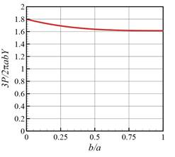
Elastic Limit: The stresses in both solids are identical, and therefore yield occurs first in the solid with the lower yield stress.  The graph below shows the critical load required to cause yield in a solid with Von-Mises yield criterion, and uniaxial tensile yield stress Y, based on tabular values in Johnson (1985)

 

 

 

5.4.12 Load-displacement-contact area relations for arbitrarily shaped axisymmetric contacts

 

The most important properties of general frictionless axisymmetric contacts can be calculated from simple formulas, even when full expressions for the stress and displacement fields cannot be calculated.

 

The figure above illustrates the problem to be solved. Assume that:

 

1. The two contacting solids have elastic constants $E_1,{\nu }_1,E_2,{\nu }_2$.  Define an effective elastic constant as

$E^{*}={\left\{{\displaystyle \frac{1-{\nu }_1^2}{E_1}+{\displaystyle \frac{1-{\nu }_2^2}{E_2}}}\right\}}^{-1}$

 

2. The surfaces of the two solids are axisymmetric near the point of initial contact.

 

3. When the two solids just touch, the gap between them can be described by a monotonically increasing function $g(r)$, where r is the distance from the point of initial contact. For example, a cone contacting a flat surface would have $g(r)=r/\tan \beta$, where $\beta$ is the cone angle; a sphere contacting a flat surface could be approximated using $g(r)=r^2/D$ where D  is the sphere diameter.  In the following we will use $g^{\prime }(r)\equiv dg/dr$

 

4. The two solids are pushed into contact by a force P.   The solids deform so as to make contact over a circular region with radius a, and move together by a distance h as the load is applied.

 

5. The relationship between h and the contact radius a will be specified by a functional relationship of the form h=H(a).   The derivative of this function with respect to its argument will be denoted by $H^{\prime }(a)$

 

These quantities are related by the following formulas:

 

1. Approach as a function of contact radius

$H(a)=a{\displaystyle \underset{0}{\overset{a}{\int }}{\displaystyle \frac{g^{\prime }(\xi )}{\sqrt{a^2-{\xi }^2}}}}d\xi$

 

2. Applied force as a function of contact radius

$P=2E^{*}\left(aH(a)-{\displaystyle \underset{0}{\overset{a}{\int }}H(\xi )d\xi }\right)$

 

3. Contact stiffness

${\displaystyle \frac{dP}{dh}=2E^{*}a}$

 

4. Contact pressure distribution 

$p(r)={\displaystyle \frac{E^{*}}{\pi }{\displaystyle \underset{r}{\overset{a}{\int }}{\displaystyle \frac{H^{\prime }(\xi )}{\sqrt{{\xi }^2-r^2}}}}d\xi }$

 

 

Once these formulas have been evaluated for a given contact geometry the results can be combined to determine other relationships, such as contact radius or stiffness as a function of load or approach h.