5.5 Solutions to dynamic problems for isotropic linear elastic solids

 

Dynamic problems are even more difficult to solve than static problems.   Nevertheless, analytical solutions have been determined for a wide range of important problems.  There is not space here to do justice to the subject, but a few solutions will be listed to give a sense of the general features of solutions to dynamic problems.

 

 

 

5.5.1 Love potentials for dynamic solutions for isotropic solids

 

In this section we outline a general potential representation for 3D dynamic linear elasticity problems.  The technique is similar to the 3D  Papkovich-Neuber representation for static solutions outlined in Section 5.4.

 

The figure shows a generic problem of interest.  Assume that

 

· The solid has Young’s modulus E, mass density ${\rho }_0$ and Poisson’s ratio $\nu$.

 

· Define longitudinal and shear wave speeds (see Sect 4.4.5)

$c_L=\sqrt{{\displaystyle \frac{E(1-\nu )}{{\rho }_0(1+\nu )(1-2\nu )}}}{c}_s=\sqrt{{\displaystyle \frac{E}{2(1+\nu ){\rho }_0}}}$

 

·         Body forces are neglected (a rather convoluted procedure exists for problems involving body force)

 

·         The solid is assumed to be at rest for t<0

 

·         Part of the boundary ${\partial }_{1}R$ is subjected to time dependent prescribed displacements $u_i^{*}$

 

·         A second part of the boundary ${\partial }_{2}R$ is subjected to prescribed tractions $t_i^{*}$

 

 

The procedure can be summarized as follows:

 

1. Find a vector function ${\Psi }_i(x_1,x_2,x_3,t)$  and a scalar function $\varphi (x_1,x_2,x_3,t)$ which satisfy

${\displaystyle \frac{\partial {\Psi }_i}{\partial x_i}=0{\displaystyle \frac{{\partial }^2{\Psi }_i}{\partial x_j\partial x_j}={\displaystyle \frac{1}{c_s^2}{\displaystyle \frac{{\partial }^2{\Psi }_i}{\partial t^2}{\displaystyle \frac{{\partial }^2\varphi }{\partial x_k\partial x_k}={\displaystyle \frac{1}{c_L^2}{\displaystyle \frac{{\partial }^2\varphi }{\partial t^2}}}}}}}}$

as well as boundary conditions

$\begin{array}{l}{\displaystyle \frac{\partial \varphi }{\partial x_i}+{\in }_{ijk}{\displaystyle \frac{\partial {\Psi }_k}{\partial x_j}=u_i^{*}\text{on }{S}_1}}\\ {\displaystyle \frac{{\partial }^2\varphi }{\partial x_i\partial x_j}{n}_j+{\displaystyle \frac{1}{2}\left({\in }_{ilk}{\displaystyle \frac{{\partial }^2{\Psi }_k}{\partial x_l\partial x_j}+{\in }_{jlk}{\displaystyle \frac{{\partial }^2{\Psi }_k}{\partial x_l\partial x_i}}}\right)n_j+{\displaystyle \frac{\nu n_i}{1-2\nu }{\displaystyle \frac{{\partial }^2\varphi }{\partial x_k\partial x_k}={\displaystyle \frac{(1+\nu )}{E}{t}_i^{*}\text{on }{S}_2}}}}}\end{array}$

and initial conditions ${\Psi }_i=\varphi =0$.

 

2. Calculate displacements from the formula

$u_i={\displaystyle \frac{\partial \varphi }{\partial x_i}+{\in }_{ijk}{\displaystyle \frac{\partial {\Psi }_k}{\partial x_j}}}$

 

3. Calculate stresses from the formula

${\displaystyle \frac{(1+\nu )}{E}{\sigma }_{ij}={\displaystyle \frac{{\partial }^2\varphi }{\partial x_i\partial x_j}+{\displaystyle \frac{1}{2}\left({\in }_{ilk}{\displaystyle \frac{{\partial }^2{\Psi }_k}{\partial x_l\partial x_j}+{\in }_{jlk}{\displaystyle \frac{{\partial }^2{\Psi }_k}{\partial x_l\partial x_i}}}\right)+{\displaystyle \frac{\nu {\delta }_{ij}}{1-2\nu }{\displaystyle \frac{{\partial }^2\varphi }{\partial x_k\partial x_k}}}}}}$

 

You can easily show that this solution satisfies the equations of motion for an elastic solid, by substituting the formula for displacements into the Cauchy-Navier equation

${\displaystyle \frac{1}{1-2\nu }{\displaystyle \frac{{\partial }^2{u}_k}{\partial x_k\partial x_i}+{\displaystyle \frac{{\partial }^2{u}_i}{\partial x_k\partial x_k}={\displaystyle \frac{{\rho }_0}{\mu }{\displaystyle \frac{{\partial }^2{u}_i}{\partial t^2}}}}}}$

The details are left as an exercise.   More importantly, one can also show that the representation is complete, i.e. all dynamic solutions can be derived from some appropriate combination of potentials.

 

 

 

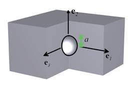
5.5.2 Pressure suddenly applied to the surface of a spherical cavity in an infinite solid

 

The figure below shows a spherical cavity with radius a in an infinite elastic solid with Young’s modulus E and Poisson’s ratio $\nu$.  The solid is at rest for t<0.   A time t=0, a pressure p is applied to the surface of the hole, and thereafter held fixed.

 

 

The solution is generated by Love potentials

${\Psi }_i=0\varphi =-{\displaystyle \frac{(1+\nu )a^{3}p}{2ER}\left\{1-\sqrt{2(1-\nu )}{e}^{-\alpha s}\sin \left(\beta s+\gamma \right)\right\}}$

where

$\begin{array}{l}\alpha ={\displaystyle \frac{1-2\nu }{1-\nu }\beta ={\displaystyle \frac{\sqrt{1-2\nu }}{1-\nu }\gamma ={\cot }^{-1}\sqrt{1-2\nu }R=\sqrt{x_k{x}_k}}}\\ s=\left\{\begin{array}{c}(c_{L}t-R+a)/aR-a<c_{L}t\\ 0R-a>c_{L}t\end{array}\right.\end{array}$

The displacements and stresses follow as

$\begin{array}{l}{u}_i={\displaystyle \frac{(1+\nu )a^{3}p{x}_i}{2E{R}^3}\left\{1-\sqrt{2(1-\nu )}{e}^{-\alpha s}\sin \left(\beta s+\gamma \right)\left({\displaystyle \frac{\beta R\cot \left(\beta s+\gamma \right)-\alpha R}{a}+1}\right)\right\}}\\ {\sigma }_{ij}=-{\displaystyle \frac{a^{3}p}{2R^3}\left(3{\displaystyle \frac{x_i{x}_j}{R^2}-{\delta }_{ij}}\right)\left\{1-\sqrt{2(1-\nu )}{e}^{-\alpha s}\sin \left(\beta s+\gamma \right)\left({\displaystyle \frac{\beta R\cot \left(\beta s+\gamma \right)-\alpha R}{a}+1}\right)\right\}}\\ +{\displaystyle \frac{ap}{2R}\left({\displaystyle \frac{x_i{x}_j}{R^2}+{\displaystyle \frac{\nu {\delta }_{ij}}{1-2\nu }}}\right)\sqrt{2(1-\nu )}{e}^{-\alpha s}\sin (\beta s+\gamma )\left\{\left({\alpha }^2-{\beta }^2\right)-2\beta \alpha \cot (\beta s+\gamma )\right\}}\end{array}$

The radial and hoop stresses at several time intervals are plotted below.

 

 

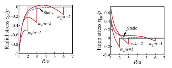
Observe that

 

1. A wave front propagates out from the cavity at the longitudinal wave speed $c_L$;

 

2. Unlike the simple 2D wave problems discussed in Section 4.4, the stress is not constant behind the front.  Instead, each point in the solid experiences a damped oscillation in displacement and stress that eventually decays to the static solution;

 

3. Both the radial and hoop stress reverse sign as the wave passes by.  For this reason dynamic loading can cause failures to occur in very unexpected places;

 

4. The maximum stress induced by dynamic loading substantially exceeds the static solution. 

 

 

 

5.5.3 Rayleigh waves

 

A Rayleigh wave is a special type of wave which propagates near the surface of an elastic solid.  Assume that

 

· The solid is an isotropic, linear elastic material with Young’s modulus $E$, Poisson’s ratio $\nu$ and mass density ${\rho }_0$

 

· The solid has shear wave speed  $c_s$ and longitudinal wave speed $c_L$

 

· The surface is free of tractions

 

· A Rayleigh wave with wavelength $\lambda$ propagates in the $x_1$ direction, as shown below

 

 

 

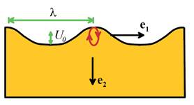
The displacement and stress due can be derived from Love potentials

$\begin{array}{l}\varphi ={\displaystyle \frac{U_0(k^2+{\beta }_T^2)}{{\beta }_L(k^2-{\beta }_T^2)}\exp \left(-{\beta }_L{x}_2\right)\exp \left(ik(x_1-c_{R}t)\right)}\\ {\Psi }_k={\displaystyle \frac{2ik{U}_0{\delta }_{k3}}{(k^2-{\beta }_T^2)}\exp \left(-{\beta }_T{x}_2\right)\exp \left(ik(x_1-c_{R}t)\right)}\end{array}$

where $i=\sqrt{-1}$, $U_0$ is the amplitude of the vertical displacement at the free surface, $k=2\pi /\lambda$ is the wavenumber

${\beta }_L=k\sqrt{1-c_R^2/c_L^2}{\beta }_T=k\sqrt{1-c_R^2/c_s^2}$

and $c_R$ is the Rayleigh wave speed, which is the positive real root of

${\left(2-{\displaystyle \frac{c_R^2}{c_s^2}}\right)}^2-4{\left(1-{\displaystyle \frac{(1-2\nu )}{2(1-\nu )}{\displaystyle \frac{c_R^2}{c_s^2}}}\right)}^{1/2}{\left(1-{\displaystyle \frac{c_R^2}{c_s^2}}\right)}^{1/2}=0$

This equation can easily be solved for $c_R/c_s$ with a symbolic manipulation program, which will most likely return 6 roots.  The root of interest lies in the range $0.65<c_R/c_s<1$ for $-1<\nu <0.5$. The solution can be approximated by $c_R/c_s=0.875-0.2\nu -0.05{(\nu +0.25)}^3$ with an error of less than 0.6% over the full range of Poisson ratio.

 

The nonzero components of displacement and stress follow as

$\begin{array}{l}{u}_1={\displaystyle \frac{U_{0}ik}{(k^2-{\beta }_T^2){\beta }_L}\exp \left(ik(x_1-c_{R}t)\right)\left\{(k^2+{\beta }_T^2)\exp \left(-{\beta }_L{x}_2\right)-2{\beta }_L{\beta }_T\exp \left(-{\beta }_T{x}_2\right)\right\}}\\ u_2={\displaystyle \frac{U_0}{(k^2-{\beta }_T^2)}\exp \left(ik(x_1-c_{R}t)\right)\left\{2k^2\exp \left(-{\beta }_T{x}_2\right)-(k^2+{\beta }_T^2)\exp \left(-{\beta }_L{x}_2\right)\right\}}\end{array}$

$\begin{array}{l}{\sigma }_{11}={\displaystyle \frac{U_{0}E\exp \left(ik(x_1-c_{R}t)\right)}{(k^2-{\beta }_T^2)(1+\nu )(1-2\nu ){\beta }_L}\left\{k^2\left[\nu ({\beta }_L^2+{\beta }_T^2)-(1-\nu )(k^2+{\beta }_T^2)\right]\exp \left(-{\beta }_L{x}_2\right)\right.}\\ \left.+2k^2{\beta }_T{\beta }_L(1-2\nu )\exp \left(-{\beta }_T{x}_2\right)\right\}\\ {\sigma }_{22}={\displaystyle \frac{U_{0}E\exp \left(ik(x_1-c_{R}t)\right)}{(k^2-{\beta }_T^2)(1+\nu )(1-2\nu ){\beta }_L}\left\{(k^2+{\beta }_T^2)\left[(1-\nu ){\beta }_L^2-\nu k^2\right]\exp \left(-{\beta }_L{x}_2\right)\right.}\\ \left.-2k^2{\beta }_T{\beta }_L(1-2\nu )\exp \left(-{\beta }_T{x}_2\right)\right\}\\ {\sigma }_{12}={\displaystyle \frac{i{U}_{0}kE(k^2+{\beta }_T^2)}{(k^2-{\beta }_T^2)(1+\nu )}\exp \left(ik(x_1-c_{R}t)\right)\left\{\exp \left(-{\beta }_T{x}_2\right)-\exp \left(-{\beta }_L{x}_2\right)\right\}}\end{array}$

You can use either the real or imaginary part of these expressions for the displacement and stress fields (they are identical, except for a phase difference). Of course, if you choose to take the real part of one of the functions, you must take the real part for all the others as well. Note that substituting $x_2=0$ in the expression for ${\sigma }_{22}$ and setting ${\sigma }_{22}=0$ yields the equation for the Rayleigh wave speed, so the boundary condition ${\sigma }_{22}=0$ is satisfied.  The variations with depth of stress amplitude and displacement amplitude are plotted below.

 

Important features of this solution are

 

1. The wave is confined to a layer near the surface with thickness about twice the wavelength. 

 

2. The horizontal and vertical components of displacement are 90 degrees out of phase.  Material particles therefore describe elliptical orbits as the wave passes by.

 

3. The speed of the wave is independent of its wavelength $–$ that is to say, the wave is non-dispersive.

 

4. Rayleigh waves are exploited in a range of engineering applications, including surface acoustic wave devices; touch sensors; and miniature linear motors.  They are also observed in earthquakes, although these waves are observed to be dispersive, because of density variations of the earth’s surface.

 

 

 

5.5.4 Love waves

 

Love waves are a second form of surface wave, somewhat similar to Rayleigh waves, which propagate through a thin elastic layer bonded to the surface of an elastic half space, as shown in the figure Love waves involve motion perpendicular to the plane of the figure.

 

Assume that

 

· The layer has thickness H, shear modulus ${\mu }_f$ and shear wave speed $c_{sf}$

 

· The substrate has shear modulus $\mu$ and shear wave speed $c_s$

 

· The wave speeds satisfy $c_{sf}<c_s$ 

 

The displacement and stress associated with a harmonic Love wave with wavelength $\lambda$ which propagates in the $x_1$ direction can be derived from Love potentials

${\Psi }_k=\left\{\begin{array}{c}{\displaystyle \frac{-U_0{\mu }_f\gamma {\delta }_{k1}\exp (-\beta x_2)}{\beta \left(\mu \beta \sin \gamma H+{\mu }_f\gamma \cos \gamma H\right)}\exp (ik(x_1-ct))x_2>0}\\ {\displaystyle \frac{U_0{\delta }_{k1}\left(\mu \beta \cos (\gamma x_2)+{\mu }_f\gamma \sin (\gamma x_2)\right)}{\gamma \left(\mu \beta \sin \gamma H+{\mu }_f\gamma \cos \gamma H\right)}\exp (ik(x_1-ct))x_2<0}\end{array}\right.$

where $U_0$ is the amplitude of the vertical displacement at the free surface, $k=2\pi /\lambda$ is the wavenumber;

$\beta =k\sqrt{1-c^2/c_s^2}\gamma =k\sqrt{c^2/c_{sf}^2-1}$

and $c$ is the wave speed (also known as the phase velocity) of the wave, which is given by the positive real roots of

$\tan \left\{kH\sqrt{{\displaystyle \frac{c^2}{c_{sf}^2}-1}}\right\}-{\displaystyle \frac{\mu }{{\mu }_f}{\displaystyle \frac{\sqrt{1-c^2/c_s^2}}{\sqrt{c^2/c_{sf}^2-1}}=0}}$

 

 

This relationship is very unlike the equations for wave speeds in unbounded or semi-infinite solids, and leads to a number of counter-intuitive results.   Note that

 

1. The wave speed depends on its wavelength.  A wave with these properties is said to be dispersive, because a pulse consisting of a spectrum of harmonic waves tends to spread out;

 

2. The wave speed is always faster than the shear wave speed of the layer, but less than the wave speed in the substrate;

 

3. If a wave with wavenumber $k_0$ propagates at speed c, then waves with wavenumber $k_n=k_0+n\pi /H\sqrt{c^2/c_{sf}^2-1}$ where n is any integer, also propagate at the same speed.   These waves are associated with different propagation modes for the wave.  Each propagation mode has a characteristic displacement distribution through the thickness of the layer, as discussed below.

 

4. A wave with a particular wave number can propagate at several different speeds, depending on the mode.  The number of modes that can exist at a particular wave number increases with the wave number.  You can see this in the plot of wave speed $–$v- wave number below.

 

 

5. Dispersive wave motion is often characterized by relating the frequency of the wave to its wave number, rather than by relating wave speed to wave number.   The (angular) frequency is related to wave number and wave speed by the usual formula $\omega =ck$.  Substituting this result into the equation for wave speed yields the Dispersion Relation for the wave

$\tan \left\{\sqrt{{(\omega H/c_{sf})}^2-{(kH)}^2}\right\}-{\displaystyle \frac{\mu }{{\mu }_f}{\displaystyle \frac{\sqrt{{(kH)}^2-{(\omega H/c_s)}^2}}{\sqrt{{(\omega H/c_{sf})}^2-{(kH)}^2}}=0}}$

 

The nonzero displacement component is

$u_3=\left\{\begin{array}{c}{\displaystyle \frac{-U_0\left(\mu \beta \sin (\gamma x_2)-{\mu }_f\gamma \cos (\gamma x_2)\right)}{\left(\mu \beta \sin \gamma H+{\mu }_f\gamma \cos \gamma H\right)}\exp (ik(x_1-ct))x_2<0}\\ {\displaystyle \frac{U_0{\mu }_f\gamma \exp (-\beta x_2)}{\left(\mu \beta \sin \gamma H+{\mu }_f\gamma \cos \gamma H\right)}\exp (ik(x_1-ct))x_2>0}\end{array}\right.$

The nonzero stresses in the layer can be determined from ${\sigma }_{3i}={\mu }_f\partial u_3/\partial x_i$, but the calculation is so trivial the result will not be written out here.  The wave speed is plotted as a function of wave number in the graph below, for the particular case $\mu ={\mu }_f$, $c_s/c_{sf}=2$.   The displacement amplitude a function of depth is shown for several modes is shown below on the right.   

 

 

 

 

5.5.5 Elastic waves in waveguides

 

The surface layer discussed in the preceding section is an example of a waveguide: it is a structure which causes waves to propagate in a particular direction, as a result of the confining effect of its geometry.

 

The figure shows a much simpler example of a waveguide: it is a thin sheet of material, with thickness H and infinite length in the $x_1$ and $x_3$ directions.  The strip can guide three types of wave:

 

1. Transverse waves, which propagate in the $x_1$ direction with particle motion in the $x_3$ direction;

 

2. Flexural waves, which propagate in the $x_1$ direction with particle motion in the $x_2$ direction;

 

3. Longitudinal waves, which propagate in the $x_1$ direction with particle motion in the $x_2$ direction.

 

The solutions for cases 2 and 3 are lengthy, but the solution for case 1 is simple, and can be used to illustrate the general features of waves in waveguides.  For transverse waves:

 

1. The wave can be any member of the following family of possible displacement distributions

$u_3=U_n\left\{{\sin }^2(\pi n/2)\sin (n\pi x_2/2H)+{\cos }^2(\pi n/2)\cos (n\pi x_2/2H)\right\}\exp (ik(x_1-ct))$

where n=0,1,2…, and you can use either the real or imaginary part as the solution. This displacement represents a harmonic wave that has wavenumber $k=2\pi /\lambda$ where $\lambda$ is the wavelength in the $x_1$ direction, which propagates in the $x_1$ direction with speed c.  The variation of displacement with $x_2$ at any fixed value of $x_1$ is a standing wave with wavelength $H/n$ and angular frequency $\omega =kc$. Each value of n corresponds to a different propagation mode.

 

2. The speed of wave propagation (usually referred to as the phase velocity of the wave)  satisfies

${\displaystyle \frac{c^2}{c_s^2}={\left({\displaystyle \frac{n\pi }{2kH}}\right)}^2+1}$

 

3. The wave speeds for modes with n>0 depend on the wave number: i.e. the waves are dispersive;

 

4. There are an infinite number of possible wave speeds for each wave number.  Each wave speed is associated with a particular propagation mode n.

 

5. The formula for wave speed can be re-written as an equation relating the angular frequency $\omega =kc$ to the wave number k. 

${\left({\displaystyle \frac{\omega H}{c_s^{}}}\right)}^2={\left({\displaystyle \frac{n\pi }{2}}\right)}^2+{\left(kH\right)}^2$

This is called the dispersion relation for the wave.

 

6. Dispersive waves have a second wave speed associated with them called the Group Velocity.  This wave speed is defined as the slope of the dispersion relation $c_g=d\omega /dk$ (in contrast, the phase velocity is $c=\omega /k$ ).  For the waveguide considered here

$c_g={\displaystyle \frac{d\omega }{dk}={\displaystyle \frac{c_{s}kH}{\sqrt{{(n\pi /2)}^2+k^2{H}^2}}}}$

The group velocity, like the phase velocity, depends on the propagation mode and the wave number.  The group velocity has two physical interpretations (i) it is the speed at which the energy in a harmonic wave propagates along the waveguide; and (ii) it is the propagation speed of an amplitude modulated wave of the form

$\begin{array}{l}{u}_3=U_0\cos (\Delta k{x}_1-\Delta \omega t)\sin (k{x}_1-\omega t)\\ =U_0\left\{\sin \left[(k+\Delta k)x_1-(\omega +\Delta \omega )t\right]+\sin \left[(k-\Delta k)x_1-(\omega -\Delta \omega )t\right]\right\}/2\end{array}$

where $\Delta k<<k$ and $\Delta \omega <<\omega$ are the wave number and frequency of the modulation, and $k,\omega$ are the wavenumber and frequency of the carrier wave.   The carrier wave propagates with speed $c$, while the modulation (which can be regarded as a `group’ of wavelets) propagates at speed $c_g$.  Note that for a non-dispersive wave, the group and phase velocities are the same.