5.6 Energy methods for solving static linear elasticity problems

 

You may recall that energy methods can often be used to simplify complex problems.  For example, to find the equilibrium configuration of a discrete system, you would begin by identifying a suitable set of generalize coordinates $q_i$, and then express the potential energy in terms of these: $V(q_i)$.  The equilibrium values of the generalized coordinates could then be determined from the condition that the potential energy is stationary at equilibrium: this gives a set of equations $\partial V/\partial q_i=0$ that could be solved for $q_i$.

 

In this section, we will develop an analogous procedure for solving boundary value problems in linear elasticity.  Our generalized coordinates will be the displacement field $u_i(x)$.  We will find an expression for the potential energy of an elastic solid in terms of $u_i$, and then show that the potential energy is stationary if the solid is in equilibrium.  We will find, further, that the potential energy is not only stationary, but is always a minimum, implying that equilibrium configurations in linear elasticity problems are always stable.  (This is because the approximations made in setting up the equations of linear elasticity preclude any possibility of buckling).  This principle will be referred to as the Principle of Minimum Potential Energy. 

 

The main application of the principle is to generate approximate solutions to linear elastic boundary value problems.  Indeed, the principle will form the basis of the Finite Element Method in linear elasticity.

 

 

 

5.6.1 Definition of the potential energy of a linear elastic solid under static loading

 

In the following, we consider a generic static boundary value problem in linear elasticity, as shown in the figure.

 

As always, we assume that we are given:

 

1. The shape of the solid in its unloaded condition $R$

 

2. The initial stress field in the solid (we will take this to be zero)

 

3. The elastic constants for the solid $C_{ijkl}$ and its mass density ${\rho }_0$

 

4. The thermal expansion coefficients for the solid, and temperature change from the initial configuration $\Delta T$

 

5. A body force distribution $b$ (per unit mass) acting on the solid

 

6. Boundary conditions, specifying displacements $u^{*}(x)$ on a portion ${\partial }_{1}R$ or tractions on a portion ${\partial }_{2}R$ of the boundary of R

 

 

Kinematically Admissible Displacement Fields

 

A ‘kinematically admissible displacement field’ $v_i(x)$ is any displacement field with the following properties:

 

1. $v_i$ is continuous everywhere within the solid

 

2. $v_i$ is differentiable everywhere within the solid, so that a strain field may be computed as

${\widehat{\epsilon }}_{ij}={\displaystyle \frac{1}{2}\left({\displaystyle \frac{\partial v_i}{\partial x_j}+{\displaystyle \frac{\partial v_j}{\partial x_i}}}\right)}$

 

3. $v_i$ satisfies boundary conditions anywhere that displacements are prescribed, i.e. $v(x)=u^{*}(x)$ on the portion ${\partial }_{1}R$ on the boundary.

 

 

Note that v is not necessarily the actual displacement in the solid $–$ it is just an arbitrary displacement field which satisfies any displacement boundary conditions.  You can think of it as a possible displacement field that the solid could adopt.  Out of all these possible displacement fields, it will actually select the one that minimizes the potential energy.

 

The kinematically admissible displacement field can also be thought of as a system of generalized coordinates in the context of analytical mechanics.  Recall that, to use a set of generalized coordinates in Lagranges equations, you must make sure that the system of coordinates satisfies all the constraints.  Similarly, to be admissible, our displacement field must satisfy constraints on the boundary. 

 

 

Definition of Potential Energy of an Elastic Solid

 

Next, we will define the potential energy of a solid.  The definition may look a bit strange, because it seems to give different values for potential energy depending on whether it is subjected to prescribed forces or displacements.  This is true.  But who cares, as long as the definition is useful?

 

For any kinematically admissible displacement field v, the potential energy is

$V(v)={\displaystyle \underset{V}{\int }U(v)}dV-{\displaystyle \underset{V}{\int }{\rho }_0{b}_i{v}_i}dV-{\displaystyle \underset{{\partial }_{2}R}{\int }{t}_i{v}_{i}dA}$

where

$U(v)={\displaystyle \frac{1}{2}{C}_{ijkl}\left({\widehat{\epsilon }}_{ij}-{\alpha }_{ij}\Delta T\right)\left({\widehat{\epsilon }}_{kl}-{\alpha }_{kl}\Delta T\right)}$

is the strain energy density associated with the kinematically admissible displacement field. You can interpret the three terms in the formula for V as the strain energy stored inside the solid; the work done by body forces; and the work done by surface tractions. For the particular case of an isotropic material, with $\Delta T=0$, we see that

$U(v)={\displaystyle \frac{E}{2\left(1+\nu \right)}\left({\widehat{\epsilon }}_{ij}{\widehat{\epsilon }}_{ij}+{\displaystyle \frac{\nu }{1-2\nu }{\widehat{\epsilon }}_{kk}{\widehat{\epsilon }}_{mm}}\right)}$

 

 

 

5.6.2 The principle of stationary and minimum potential energy.

 

Let v be any kinematically admissible displacement field.  Let u be the actual displacement field $–$ i.e. the one that satisfies the equilibrium equations within the solid as well as all the boundary conditions.  We will show the following:

 

1. V(v) is stationary (i.e. a local minimum, maximum or inflexion point) for v=u.

 

2. V(v) is a global minimum for v=u.

 

 

As a preliminary step, recall that the actual displacement field satisfies the following equations

$\begin{array}{l}{\epsilon }_{ij}={\displaystyle \frac{1}{2}\left({\displaystyle \frac{\partial u_i}{\partial x_j}+{\displaystyle \frac{\partial u_j}{\partial x_i}}}\right)}\\ {\sigma }_{ij}=C_{ijkl}({\epsilon }_{kl}-{\alpha }_{kl}\Delta T)\\ {\displaystyle \frac{\partial {\sigma }_{ij}}{\partial x_i}+{\rho }_0{b}_j=0}\\ u_i=u_i^{*}\text{on}{\partial }_{1}R\\ {\sigma }_{ij}{n}_i=t_j^{*}\text{on}{\partial }_{2}R\end{array}$

Next, re-write the kinematically admissible displacement field in terms of u as

$v_i=u_i+\delta u_i$

where $\delta u_i$ is the difference between the kinematically admissible field and the correct equilibrium field.  Observe that

$\begin{array}{l}{v}_i=u_i^{*}{u}_i=u_i^{*}\text{on }{\partial }_{1}R\\ \Rightarrow \delta u_i=0\text{on }{\partial }_{1}R\end{array}$

i.e. the difference between the kinematically admissible field and the actual field is zero wherever displacements are prescribed.

 

Now, note that $V(v)$ can be expressed in terms of $u_i$ and $\delta u_i$ as

$V\left(u+\delta u\right)=V(u)+\delta V+{\displaystyle \frac{1}{2}{\delta }^{2}V}$

where

$\begin{array}{l}\delta V={\displaystyle \underset{V}{\int }{C}_{ijkl}\left({\epsilon }_{ij}-{\alpha }_{ij}\Delta T\right)\delta {\epsilon }_{kl}dV}-{\displaystyle \underset{V}{\int }{b}_i\delta u_i}dV-{\displaystyle \underset{{\partial }_{2}R}{\int }{t}_i\delta u_{i}dA}\\ {\delta }^{2}V={\displaystyle \underset{V}{\int }{C}_{ijkl}\delta {\epsilon }_{ij}\delta {\epsilon }_{kl}}\\ {\epsilon }_{ij}={\displaystyle \frac{1}{2}\left({\displaystyle \frac{\partial u_i}{\partial x_j}+{\displaystyle \frac{\partial u_j}{\partial x_i}}}\right)\delta {\epsilon }_{ij}={\displaystyle \frac{1}{2}\left({\displaystyle \frac{\partial \delta u_i}{\partial x_j}+{\displaystyle \frac{\partial \delta u_j}{\partial x_i}}}\right)}}\end{array}$

To see this, simply substitute into the definition of the potential energy

$\begin{array}{l}V(v)={\displaystyle \underset{V}{\int }U(u+\delta u)}dV-{\displaystyle \underset{V}{\int }{b}_i(u_i+\delta u_i)}dV-{\displaystyle \underset{{\partial }_{2}R}{\int }{t}_i(u_i+\delta u_i)dA}\\ ={\displaystyle \underset{V}{\int }{\displaystyle \frac{1}{2}{C}_{ijkl}\left({\epsilon }_{ij}-{\alpha }_{ij}\Delta T+\delta {\epsilon }_{ij}\right)\left({\epsilon }_{kl}-{\alpha }_{kl}\Delta T+\delta {\epsilon }_{kl}\right)dV}}-{\displaystyle \underset{V}{\int }{b}_i(u_i+\delta u_i)}dV-{\displaystyle \underset{{\partial }_{2}R}{\int }{t}_i(u_i+\delta u_i)dA}\end{array}$

Multiply everything out and use the condition that $C_{ijkl}=C_{klij}$ to get the result stated.

 

Now, to show that $V(v)$ is stationary at v=u, we need to show that $\delta V=0$.  This means that, if we add any small change $\delta u$ to the actual displacement field u, the change in potential energy will be zero, to first order in $\delta u$.

 

To show this, note that

$C_{ijkl}\left({\epsilon }_{ij}-{\alpha }_{ij}\Delta T\right)={\sigma }_{kl}$

Next, note that

${\sigma }_{kl}\delta {\epsilon }_{kl}={\sigma }_{kl}{\displaystyle \frac{1}{2}\left({\displaystyle \frac{\partial \delta u_k}{\partial x_l}+{\displaystyle \frac{\partial \delta u_l}{\partial x_k}}}\right)={\displaystyle \frac{1}{2}{\sigma }_{lk}{\displaystyle \frac{\partial \delta u_k}{\partial x_l}+{\displaystyle \frac{1}{2}{\sigma }_{kl}{\displaystyle \frac{\partial \delta u_l}{\partial x_k}={\sigma }_{kl}{\displaystyle \frac{\partial \delta u_l}{\partial x_k}}}}}}}$

where we have used the fact that ${\sigma }_{kl}={\sigma }_{lk}$ (angular momentum balance).  Rewrite this as

${\sigma }_{ij}{\displaystyle \frac{\partial \delta u_j}{\partial x_i}={\displaystyle \frac{\partial }{\partial x_i}\left({\sigma }_{ij}\delta u_j\right)-{\displaystyle \frac{\partial {\sigma }_{ij}}{\partial x_i}\delta u_j}}}$

Substitute back into the expression for $\delta V$ and rearrange to see that

$\delta V={\displaystyle \underset{V}{\int }{\displaystyle \frac{\partial }{\partial x_i}\left({\sigma }_{ij}\delta u_j\right)dV}}-{\displaystyle \underset{V}{\int }\left({\displaystyle \frac{\partial {\sigma }_{ij}}{\partial x_i}+{\rho }_0{b}_j}\right)\delta u_j}dV-{\displaystyle \underset{{\partial }_{2}R}{\int }{t}_i\delta u_{i}dA}$

Now, recall the equations of equilibrium

${\displaystyle \frac{\partial {\sigma }_{ij}}{\partial x_i}+{\rho }_0{b}_j=0}$

so that the second term vanishes.  Apply the divergence theorem to express the first integral as a surface integral

${\displaystyle \underset{V}{\int }{\displaystyle \frac{\partial }{\partial x_i}\left({\sigma }_{ij}\delta u_j\right)dV={\displaystyle \underset{A}{\int }{\sigma }_{ij}\delta u_j}}}{n}_{i}dA$

Recall that $\delta u_i=0\text{on }{\partial }_{1}R$, and note that

${\displaystyle \underset{A}{\int }dA}={\displaystyle \underset{{\partial }_{1}R}{\int }dA}+{\displaystyle \underset{{\partial }_{2}R}{\int }dA}$

because either tractions or displacements (but not both) must be prescribed on every point on the boundary. 

 

Therefore

${\displaystyle \underset{V}{\int }{\displaystyle \frac{\partial }{\partial x_i}\left({\sigma }_{ij}\delta u_j\right)dV={\displaystyle \underset{A}{\int }{\sigma }_{ij}\delta u_j}}}{n}_{i}dA={\displaystyle \underset{{\partial }_{1}R}{\int }{\sigma }_{ij}{n}_i\delta u_{j}dA}+{\displaystyle \underset{{\partial }_{2}R}{\int }{\sigma }_{ij}{n}_i\delta u_{j}dA}={\displaystyle \underset{{\partial }_{2}R}{\int }{\sigma }_{ij}{n}_i\delta u_{j}dA}$

Finally, recall that

${\sigma }_{ij}{n}_i=t_j\text{on }{\partial }_{2}R$

and substitute back into the expression for $\delta V$ to see that

$\delta V={\displaystyle \underset{{\partial }_{2}R}{\int }\left({\sigma }_{ji}{n}_j-t_i\delta u_i\right)dA}=0$

This proves that V(v) is stationary at v=u, as stated.

 

Finally, we wish to show that V(v) is a minimum at v=u.  This is easy.  Note that we have proved that

$\begin{array}{l}V\left(v\right)=V(u)+{\displaystyle \frac{1}{2}{\delta }^{2}V}\\ {\delta }^{2}V={\displaystyle \underset{V}{\int }{C}_{ijkl}\delta {\epsilon }_{ij}\delta {\epsilon }_{kl}}\end{array}$

Note that

${\displaystyle \frac{1}{2}{C}_{ijlk}\delta {\epsilon }_{kl}\delta {\epsilon }_{ij}}$

is the strain energy density associated with a strain $\delta {\epsilon }_{ij}$.  Strain energy density must always be positive or zero, so that

$V\left(v\right)\ge V(u)$

 

 

 

5.6.3 Uniaxial compression of a cylinder solved by energy methods

 

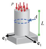Consider a cylindrical bar subjected to a uniform pressure p on one end, and supported on a rigid, frictionless base, as shown in the figure.  Neglect temperature changes.  Determine the displacement field in the bar.

 

We will solve this problem using energy methods.  We will guess a displacement field of the form

$v_1={\lambda }_1{x}_1,v_2=\lambda {}_2{x}_2{v}_3={\lambda }_3{x}_3$

This satisfies the boundary conditions on the bottom face of the cylinder, so it is a kinematically admissible displacement field.  The coefficients ${\lambda }_i$ are to be determined, by minimizing the potential energy.  The strains follow as

${\epsilon }_{11}={\lambda }_1{\epsilon }_{22}={\lambda }_2{\epsilon }_{33}={\lambda }_3$

with all other strain components zero.  The strain energy density is

$U={\displaystyle \frac{E}{2\left(1+\nu \right)}\left\{{\lambda }_1^2+{\lambda }_2^2+{\lambda }_3^2+{\displaystyle \frac{\nu }{1-2\nu }{\left({\lambda }_1+{\lambda }_2+{\lambda }_3\right)}^2}\right\}}$

The boundary conditions are

 

1. On the bottom of the cylinder $v_2=0,t_1=t_3=0\Rightarrow v_i{t}_i=0$

 

2. On the sides of the cylinder, $t_i=0\Rightarrow v_i{t}_i=0$ 

 

3. On the top of the cylinder $v_2(L)={\lambda }_{2}L{t}_2=-p,t_1=t_3=0\Rightarrow v_i{t}_i=-p{\lambda }_{2}L$

 

 

Substitute into the expression for strain energy density to see that

$\begin{array}{l}V(v)={\displaystyle \underset{V}{\int }{\displaystyle \frac{E}{2\left(1+\nu \right)}\left\{{\lambda }_1^2+{\lambda }_2^2+{\lambda }_3^2+{\displaystyle \frac{\nu }{1-2\nu }{\left({\lambda }_1+{\lambda }_2+{\lambda }_3\right)}^2}\right\}dV-{\displaystyle \underset{A}{\int }{\lambda }_{2}L(-p)}}}\\ ={\displaystyle \frac{ALE}{2\left(1+\nu \right)}\left\{{\lambda }_1^2+{\lambda }_2^2+{\lambda }_3^2+{\displaystyle \frac{\nu }{1-2\nu }{\left({\lambda }_1+{\lambda }_2+{\lambda }_3\right)}^2}\right\}+A{\lambda }_{2}Lp}\end{array}$

Now, the actual displacement field minimizes V.  This requires

${\displaystyle \frac{\partial V}{\partial {\lambda }_1}={\displaystyle \frac{\partial V}{\partial {\lambda }_2}={\displaystyle \frac{\partial V}{\partial {\lambda }_3}=0}}}$

Evaluate the derivatives to see that

$\begin{array}{l}{\displaystyle \frac{ALE}{2\left(1+\nu \right)}\left\{2{\lambda }_1+{\displaystyle \frac{2\nu }{1-2\nu }\left({\lambda }_1+{\lambda }_2+{\lambda }_3\right)}\right\}=0}\\ {\displaystyle \frac{ALE}{2\left(1+\nu \right)}\left\{2{\lambda }_2+{\displaystyle \frac{2\nu }{1-2\nu }\left({\lambda }_1+{\lambda }_2+{\lambda }_3\right)}\right\}+ALp=0}\\ {\displaystyle \frac{ALE}{2\left(1+\nu \right)}\left\{2{\lambda }_3+{\displaystyle \frac{2\nu }{1-2\nu }\left({\lambda }_1+{\lambda }_2+{\lambda }_3\right)}\right\}=0}\end{array}$

It is easy to solve these equations to see that

${\lambda }_1=-p/E{\lambda }_2={\lambda }_3=\nu p/E$

 

This is, of course, the exact solution, which is reassuring.  Notice that we never had to calculate stresses or worry about equilibrium $–$ the variational principle takes care of all that for us.

 

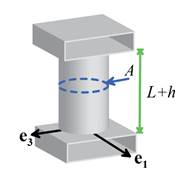Let us solve the same problem, but this time with displacement boundary conditions on the top of the cylinder, as shown in the figure.

 

The cylinder has unstretched length L and is stretched between frictionless grips to length L+h.  This time, the kinematically admissible displacement field must satisfy boundary conditions on both top and bottom surface of the cylinder.   Therefore, we choose

$v_1={\lambda }_1{x}_1,v_2=h{x}_2/L{v}_3={\lambda }_3{x}_3$

Proceeding as before, we now find that the potential energy is

$V(v)={\displaystyle \frac{ALE}{2\left(1+\nu \right)}\left\{{\lambda }_1^2+{\displaystyle \frac{h^2}{L^2}+{\lambda }_3^2+{\displaystyle \frac{\nu }{1-2\nu }{\left({\lambda }_1+{\displaystyle \frac{h}{L}+{\lambda }_3}\right)}^2}}\right\}}$

Note that this time there is no contribution to the potential energy from the tractions on the top of the cylinder, because now the displacement is prescribed there, instead of the pressure.  Minimizing the potential energy as before

$\begin{array}{l}{\displaystyle \frac{ALE}{2\left(1+\nu \right)}\left\{2{\lambda }_1+{\displaystyle \frac{2\nu }{1-2\nu }\left({\lambda }_1+{\displaystyle \frac{h}{L}+{\lambda }_3}\right)}\right\}=0}\\ {\displaystyle \frac{ALE}{2\left(1+\nu \right)}\left\{2{\lambda }_3+{\displaystyle \frac{2\nu }{1-2\nu }\left({\lambda }_1+{\displaystyle \frac{h}{L}+{\lambda }_3}\right)}\right\}=0}\end{array}$

Solve these equations to conclude that

${\lambda }_1={\lambda }_3=-\nu {\displaystyle \frac{h}{L}}$

Again, this is the exact solution.

 

 

 

5.6.4 Variational derivation of the beam equations

 

Variational methods can be used to solve boundary value problems exactly, as described in the preceding section.   The real power of variational methods, however, is to provide a systematic way to find approximate solutions to boundary value problems. 

 

We will illustrate this by re-deriving the equations governing beam bending theory using the principle of minimum potential energy.

 

 

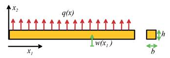
Consider a slender rod with rectangular cross section, subjected to uniform pressure q(x) on its top surface, as shown above.  Assume that the rod is an isotropic, linear elastic solid with Young’s modulus E and Poisson’s ratio $\nu$. The boundary conditions at the ends of the bar will be left unspecified for the time being.

 

 

We proceed by approximating the strain field within the bar.  The figure above shows the deflected beam. We will suppose that the strains at any given cross section are completely characterized by the local curvature of the beam, so that at a given cross section x

${\epsilon }_{11}={\displaystyle \frac{-(x_2-y_0)}{R(x_1)}{\epsilon }_{22}={\epsilon }_{33}=-\nu {\epsilon }_{11}{\epsilon }_{12}={\epsilon }_{13}={\epsilon }_{23}=0}$

Here, $y_0$ is the height of a fiber in the beam whose length is unchanged:  $y_0$ must be determined as part of the solution.

 

The displacement and strain fields are therefore completely characterized by $y_0$ and R(x). Rather than solve for R, we will approximate the curvature at x by the second derivative of the vertical deflection w, so that

${\epsilon }_{11}={\displaystyle \frac{-(x_2-y_0)}{R(x_1)}\approx -(x_2-y_0){\displaystyle \frac{d^{2}w(x_1)}{d{x}_1{}^2}}}$

 

Now, we want to find w(x) and  $y_0$ that will best approximate the actual displacement field within the bar.  We will do this by choosing w and  $y_0$ so as to minimize the potential energy of the solid.

 

Begin by computing the potential energy.  It is straightforward to show that the strain energy density is

$\varphi ={\displaystyle \frac{1}{2}E{\left\{(x_2-y_0){\displaystyle \frac{d^{2}w(x_1)}{d{x}_1{}^2}}\right\}}^2}$

Hence

$V(w,y_0)={\displaystyle \underset{0}{\overset{L}{\int }}{\displaystyle \underset{A}{\int }}}{\displaystyle \frac{1}{2}E{\left\{(x_2-y_0){\displaystyle \frac{d^{2}w(x_1)}{d{x}_1{}^2}}\right\}}^{2}dAd{x}_1-{\displaystyle \underset{0}{\overset{L}{\int }}bq(x_1)w(x_1)dx}}$

Here, we have neglected the small additional deflection of the beam surface due to ${\epsilon }_{22}$

 

We now wish to minimize V with respect to w and  $y_0$.  Do the latter first:

${\displaystyle \frac{\partial V(w,y_0)}{\partial y_0}={\displaystyle \underset{0}{\overset{L}{\int }}{\displaystyle \underset{A}{\int }}}E{\left\{(x_2-y_0){\displaystyle \frac{d^{2}w(x_1)}{d{x}_1{}^2}}\right\}}^{}dAd{x}_1=0}$

which is evidently satisfied for any w by choosing

$y_0={\displaystyle \frac{1}{A}{\displaystyle \underset{A}{\int }{x}_2}dA}$

This is the usual expression for the position of the neutral axis of a beam. We can now simplify our expression for potential energy by defining

$I={\displaystyle \frac{1}{A}{\displaystyle \underset{A}{\int }{(x_2-y_0)}^2}dA}$

so that

$V(w)={\displaystyle \underset{0}{\overset{L}{\int }}}{\displaystyle \frac{1}{2}EI{\left\{{\displaystyle \frac{d^{2}w(x_1)}{d{x}_1{}^2}}\right\}}^{2}d{x}_1-{\displaystyle \underset{0}{\overset{L}{\int }}bq(x_1)w(x_1)d{x}_1}}$

 

 

Now turn to the more difficult problem of finding w that will minimise V.  To do this, let us calculate the change in V when $w$ is changed slightly to $w+\delta w$

$\begin{array}{l}V(w+\delta w)-V(w)={\displaystyle \underset{0}{\overset{L}{\int }}}{\displaystyle \frac{1}{2}EI{\left\{{\displaystyle \frac{d^{2}w(x_1)}{d{x}_1{}^2}+{\displaystyle \frac{d^2\delta w(x_1)}{d{x}_1{}^2}}}\right\}}^{2}d{x}_1-{\displaystyle \underset{0}{\overset{L}{\int }}bq(x_1)\left\{w(x_1)+\delta w(x_1)\right\}d{x}_1}}\\ -{\displaystyle \underset{0}{\overset{L}{\int }}}{\displaystyle \frac{1}{2}EI{\left\{{\displaystyle \frac{d^{2}w(x_1)}{d{x}_1{}^2}}\right\}}^{2}d{x}_1-{\displaystyle \underset{0}{\overset{L}{\int }}bq(x_1)w(x_1)d{x}_1}}\end{array}$

Expand this out to see that

$\begin{array}{l}V(w+\delta w)-V(w)={\displaystyle \underset{0}{\overset{L}{\int }}}EI{\displaystyle \frac{d^{2}w(x_1)}{d{x}_1{}^2}{\displaystyle \frac{d^2\delta w(x_1)}{d{x}_1{}^2}d{x}_1-{\displaystyle \underset{0}{\overset{L}{\int }}bq(x_1)\delta w(x_1)d{x}_1}}}\\ +{\displaystyle \underset{0}{\overset{L}{\int }}}{\displaystyle \frac{1}{2}EI{\left\{{\displaystyle \frac{d^2\delta w(x_1)}{d{x}_1{}^2}}\right\}}^{2}d{x}_1}\end{array}$

Now, if V(w) is a minimum, then

${\displaystyle \underset{0}{\overset{L}{\int }}}EI{\displaystyle \frac{d^{2}w(x_1)}{d{x}_1{}^2}{\displaystyle \frac{d^2\delta w(x_1)}{d{x}_1{}^2}d{x}_1-{\displaystyle \underset{0}{\overset{L}{\int }}bq(x_1)\delta w(x_1)d{x}_1}=0}}$

We are none the wiser as a result of this exercise, but if we integrate the first integral by parts twice, we find that

${\left[EI{\displaystyle \frac{d^{2}w}{d{x}_1{}^2}{\displaystyle \frac{d\delta w}{d{x}_1}}}\right]}_0^L-{\left[{\displaystyle \frac{d}{d{x}_1}(EI{\displaystyle \frac{d^{2}w}{d{x}_1{}^2})\delta w}}\right]}_0^L+{\displaystyle \underset{0}{\overset{L}{\int }}}\left(EI{\displaystyle \frac{d^{4}w(x_1)}{d{x}_1{}^4}-bq(x_1)}\right)\delta wd{x}_1=0$

 

Since this is zero for any $\delta w$ we conclude that

$EI{\displaystyle \frac{d^{4}w(x_1)}{d{x}_1{}^4}-bq(x_1)=0}$

to ensure that the third term in this expression vanishes.  This gives us the required governing equation for w.  However, we still need to deal with the first two boundary terms.

 

There are several ways to prescribe boundary conditions on the ends of the beam to ensure that V is stationary.

 

1. We may prescribe w and its first derivative.  In this case the variation in $w$ must satisfy $\delta w=d\delta w/dx=0$ to ensure that w is a kinematically admissible displacement.  The boundary terms are zero under these conditions

 

2. Prescribe only the value of w. In this case we must ensure that $\delta w=0$ on the end of the beam. The  second boundary term is automatically zero.  To ensure that the first boundary term is zero we must set

${\displaystyle \frac{d^{2}w}{d{x}_1{}^2}=0}$

to ensure that V is stationary.  We know from elementary strength of materials courses that this is equivalent to the condition that the shear force vanishes on the end of the beam.

3. Prescribe only the value of $dw/dx$.  In this case, we must ensure that $d\delta w/dx=0$ so that $w+\delta w$ is a kinematically admissible displacement.  The first boundary term vanishes; while the second boundary term is zero if we choose

${\displaystyle \frac{d}{d{x}_1}\left(EI{\displaystyle \frac{d^{2}w}{d{x}_1{}^2}}\right)=0}$

This is equivalent to setting the bending moment to zero at the end of the beam.

 

Clearly, one could extend this procedure to account for tractions acting on the ends of the beam.  The details are left as an exercise.  A nice feature of the variational approach that we followed here is that the appropriate boundary conditions follow naturally from the variational principle (indeed, the boundary conditions are called `natural’ boundary conditions).  This turns out to be particularly helpful in setting up approximate theories of plates and shells, where the boundary conditions can be very difficult to determine consistently using any other method.

 

 

 

5.6.5 Energy methods for calculating stiffness

 

Energy methods can also be used to calculate an upper bound to the stiffness of a structure or a component.

A spring is an example of an elastic solid.  Recall that if you apply a force P to a spring, it deflects by an amount $\Delta$, in proportion to P.  The stiffness k is defined so that

$k=P/\Delta$

If you apply a load P to any stable elastic structure (except one which contains two or more contacting surfaces, or if the forces are too large for linear elasticity theory to be applicable), the point where you apply the load will deflect by a distance that is proportional to the applied load.  For example, for the cantilever beam shown below the end deflection is

$\Delta ={\displaystyle \frac{P{L}^3}{2E{a}^{3}b}}$

The stiffness of the beam is therefore $k=P/\Delta =2E{a}^{3}b/L^3$

 

 

To get an upper bound to the stiffness of a structure, one can merely guess its deformed shape, then apply the principle of minimum potential energy.

 

For example, for the beam problem, we might guess that the beam deforms into a circular shape, with unknown radius R, as shown below

 

 

The deflection at the end of the beam is approximately

$\Delta =R-\sqrt{R^2-L^2}\approx {\displaystyle \frac{L^2}{2R}}$

From the preceding section, we know that the potential energy of a beam is

$V(w)={\displaystyle \underset{0}{\overset{L}{\int }}}{\displaystyle \frac{1}{2}EI{\left\{{\displaystyle \frac{d^{2}w(x_1)}{d{x}_1{}^2}}\right\}}^{2}d{x}_1-{\displaystyle \underset{0}{\overset{L}{\int }}bq(x_1)w(x_1)d{x}_1}}$

Here, $q(x_1)=0$, but we need to account for the potential energy of the load P.  Recall that the potential energy of a constant force is $-P\Delta$. Recall also that $d^{2}w/d{x}^2\approx 1/R$. Thus

$V(R)={\displaystyle \underset{0}{\overset{L}{\int }}{\displaystyle \frac{1}{2}{\displaystyle \frac{EI}{R^2}}}}d{x}_1-P\Delta ={\displaystyle \frac{1}{2}{\displaystyle \frac{EI}{R^2}L-P{\displaystyle \frac{L^2}{2R}}}}$

Choose R to minimize the potential energy

${\displaystyle \frac{\partial V}{\partial R}=0\Rightarrow -{\displaystyle \frac{EI}{R^3}L+P{\displaystyle \frac{L^2}{2R^2}=0\Rightarrow R={\displaystyle \frac{2EI}{PL}}}}}$

so that

$\Delta ={\displaystyle \frac{L^2}{2R}={\displaystyle \frac{L^3}{4EI}P\Rightarrow k\le {\displaystyle \frac{4EI}{L^3}}}}$

For comparison, the exact solution is $k=3EI/L^3$