5.7 The Reciprocal Theorem and applications

 

The reciprocal theorem is a distant cousin of the principle of minimum potential energy, and is a particularly useful tool.  It is the basis for a computational method in linear elasticity called the boundary element method; it can often be used to extract information concerning solutions to a boundary value problem without having to solve the problem in detail;  and can occasionally be used to find the full solution $–$ for example, the reciprocal theorem provides a way to compute fields for arbitrarily shaped dislocation loops in an infinite solid.

 

 

 

5.7.1 Statement and proof of the reciprocal theorem

                                                      

The reciprocal theorem relates two solutions for the same elastic solid, when subjected to different loads. 

 

 

To this end, consider the following scenario

 

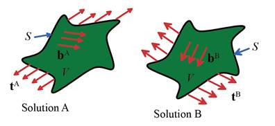
1. An elastic solid which occupies some region V with boundary S, as shown above. The outward normal to the boundary is specified by a unit vector $n$.  The properties of the solid are characterized by the tensor of elastic moduli $C_{ijkl}$ and mass density ${\rho }_0$.  The solid is free of stress when unloaded, and temperature changes are neglected.

 

2. When subjected to body forces $b^A$ (per unit mass) together with prescribed displacements $u^{*A}$ on portion $S_{1A}$ of its boundary, and tractions  $t^{*A}$ on portion $S_{2A}$, a state of static equilibrium is established in the solid with displacements, strains and stresses $u_i^A,{\epsilon }_{ij}^A,{\sigma }_{ij}^A$

 

3. When subjected to body forces $b^B$ together with prescribed displacements $u^{*B}$ on portion $S_{1B}$ of its boundary, and tractions  $t^{*B}$ on portion $S_{2B}$, the solid experiences a static state $u_i^B,{\epsilon }_{ij}^B,{\sigma }_{ij}^B$

 

 

The reciprocal theorem relates the two solutions through

${\displaystyle \underset{S}{\int }{n}_i{\sigma }_{ij}^A{u}_j^{B}dA}+{\displaystyle \underset{V}{\int }{\rho }_0{b}_i^A{u}_i^{B}dV}={\displaystyle \underset{S}{\int }{n}_i{\sigma }_{ij}^B{u}_j^{A}dA}+{\displaystyle \underset{V}{\int }{\rho }_0{b}_i^B{u}_i^{A}dV}={\displaystyle \underset{V}{\int }{\sigma }_{ij}^A{\epsilon }_{ij}^{B}dV}={\displaystyle \underset{V}{\int }{\sigma }_{ij}^B{\epsilon }_{ij}^{A}dV}$

 

 

 Derivation:

 

Start by showing that ${\sigma }_{ij}^A{\epsilon }_{ij}^B={\sigma }_{ij}^B{\epsilon }_{ij}^A$.  To see this, note that ${\sigma }_{ij}^A{\epsilon }_{ij}^B=C_{ijkl}{\epsilon }_{kl}^B{\epsilon }_{ij}^A=C_{klij}{\epsilon }_{kl}^B{\epsilon }_{ij}^A={\sigma }_{ij}^B{\epsilon }_{ij}^A$, where we have used the symmetry relation $C_{ijkl}=C_{klij}$.

 

To prove the rest, recall that

 

1. The divergence theorem requires that

${\displaystyle \underset{S}{\int }{n}_i{\sigma }_{ij}{u}_{j}dA}={\displaystyle \underset{V}{\int }{\displaystyle \frac{\partial ({\sigma }_{ij}{u}_j)}{\partial x_i}dV}}={\displaystyle \underset{V}{\int }\left({\displaystyle \frac{\partial {\sigma }_{ij}}{\partial x_i}{u}_j+{\sigma }_{ij}{\displaystyle \frac{\partial u_j}{\partial x_i}}}\right)dV}$

 

2. Any pair of strains and displacement are related by ${\epsilon }_{ij}=\left(\partial u_i/x_j+\partial u_j/x_i\right)/2$

 

3. The stress tensor is symmetric, so that ${\sigma }_{ij}\partial u_j/\partial x_i={\sigma }_{ij}(\partial u_j/\partial x_i+\partial u_i/\partial x_j)/2={\sigma }_{ij}{\epsilon }_{ij}$

 

4. Both stress states satisfy the equilibrium equation $\partial {\sigma }_{ij}/\partial x_i+{\rho }_0{b}_j=0$. Consequently, collecting together the volume integrals gives

${\displaystyle \underset{S}{\int }{n}_i{\sigma }_{ij}{u}_{j}dA}+{\displaystyle \underset{V}{\int }{\rho }_0{b}_j{u}_{j}dV}={\displaystyle \underset{V}{\int }\left(\left[{\displaystyle \frac{\partial {\sigma }_{ij}}{\partial x_i}+{\rho }_0{b}_j}\right]u_j+{\sigma }_{ij}{\epsilon }_{ij}\right)dV}={\displaystyle \underset{V}{\int }{\sigma }_{ij}{\epsilon }_{ij}dV}$

 

5. Note that this result applies to any equilibrium stress field and pair of compatible strain and displacements $–$ the stresses need not be related to the strains.  Consequently, this result can be applied to pairs of stress and displacement

${\displaystyle \underset{S}{\int }{n}_i{\sigma }_{ij}^A{u}_j^{B}dA}+{\displaystyle \underset{V}{\int }{\rho }_0{b}_i^A{u}_i^{B}dV}={\displaystyle \underset{S}{\int }{n}_i{\sigma }_{ij}^B{u}_j^{A}dA}+{\displaystyle \underset{V}{\int }{\rho }_0{b}_i^B{u}_i^{A}dV}={\displaystyle \underset{V}{\int }{\sigma }_{ij}^A{\epsilon }_{ij}^{B}dV}={\displaystyle \underset{V}{\int }{\sigma }_{ij}^B{\epsilon }_{ij}^{A}dV}$

 

 

 

5.7.2 Simple example using the reciprocal theorem

 

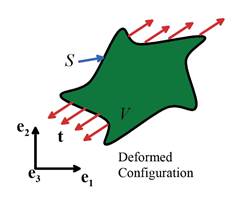
The reciprocal theorem can often be used to extract average measures of deformation or stress in an elastic solution.  As an example, consider the following problem:  An elastic solid with Young’s modulus E and Poisson’s ratio $\nu$ occupies a volume V with surface S, as shown in the figure.  The solid is subjected to a distribution of traction $t_i(x_j)$ on its surface.  The traction exerts zero resultant force and moment on the solid, i.e.

${\displaystyle \underset{S}{\int }{t}_{i}dA}=0,{\displaystyle \underset{S}{\int }{\in }_{ijk}{x}_j{t}_{k}dA}=0$

As a result, a state of static equilibrium with displacement, strain and stress $u_i,{\epsilon }_{ij},{\sigma }_{ij}$ is developed in the solid.   Show that the volume change of the solid can be calculated as

$\Delta V={\displaystyle \frac{1-2\nu }{E}{\displaystyle \underset{S}{\int }{x}_i{t}_{i}dA}}$

Derivation:

 

1. Note that if we were able to determine the full displacement field in the solid, the volume change could be calculated as

$\Delta V={\displaystyle \underset{S}{\int }{u}_i{n}_{i}dA}$

If you don’t see this result immediately on geometric grounds it can be derived by first calculating the total volume change by integrating the dilatation over the volume of the solid and then applying the divergence theorem

$\Delta V={\displaystyle \underset{V}{\int }{\epsilon }_{kk}dV}={\displaystyle \underset{V}{\int }\partial u_k/\partial x_{k}dV}={\displaystyle \underset{S}{\int }{u}_k{n}_{k}dV}$

 

2. Note that we can make one of the terms in the reciprocal theorem reduce to this formula by choosing state A to be the actual displacement, stress and strain in the solid, and choosing state B to be a uniform stress with unit magnitude ${\sigma }_{ij}^B={\delta }_{ij}$. This stress is clearly an equilibrium field, for zero body force. The corresponding strains and displacements follow as

${\epsilon }_{ij}^B={\displaystyle \frac{1-2\nu }{E}{\delta }_{ij}{u}_i^B={\displaystyle \frac{1-2\nu }{E}{x}_i+c_i+{\in }_{ijk}{\omega }_j{x}_k}}$

where $c_i$ and ${\omega }_j$ represent an arbitrary infinitesimal displacement and rotation.

 

3. Substituting into the reciprocal theorem, recalling that the stresses satisfy the boundary condition ${\sigma }_{ij}{n}_i=t_j$, and using the equilibrium equations for the traction then yields

${\displaystyle \underset{S}{\int }{n}_i{\sigma }_{ij}^{}{u}_j^{B}dA}={\displaystyle \underset{S}{\int }{n}_i{\delta }_{ij}{u}_j^{}dA}\Rightarrow \Delta V={\displaystyle \underset{S}{\int }{n}_i{u}_i^{}dA}={\displaystyle \underset{S}{\int }{t}_i\left({\displaystyle \frac{1-2\nu }{E}{x}_i+c_i+{\in }_{ijk}{\omega }_j{x}_k}\right)dA}={\displaystyle \frac{1-2\nu }{E}{\displaystyle \underset{S}{\int }{x}_i{t}_{i}dA}}$

 

 

 

5.7.3 Formulas relating internal and boundary values of field quantities

 

The reciprocal theorem also gives a useful relationship between the values of stress and displacement in the interior and on the boundary of the solid, which can be stated as follows.  Suppose that a linear elastic solid with Young’s modulus E and Poisson’s ratio $\nu$ is loaded on its boundary (with no body force) so as to induce a static equilibrium displacement, strain and stress field $u_i,{\epsilon }_{ij},{\sigma }_{ij}$ in the solid.  Define the following functions

$\begin{array}{l}{U}_i^{(k)}(x)={\displaystyle \frac{(1+\nu )}{8\pi E(1-\nu )R}\left\{{\displaystyle \frac{x_k{x}_i}{R^2}+(3-4\nu ){\delta }_{ik}}\right\}}\\ {\Sigma }_{ij}^{(k)}(x)={\displaystyle \frac{-1}{8\pi (1-\nu )R^2}\left\{{\displaystyle \frac{3x_k{x}_i{x}_j}{R^3}}\right.\left.+(1-2\nu ){\displaystyle \frac{{\delta }_{ik}{x}_j+{\delta }_{jk}{x}_i-{\delta }_{ij}{x}_k}{R}}\right\}}\\ {\Omega }_{ij}^{(kq)}(x)={\displaystyle \frac{-E}{8\pi (1-{\nu }^2)R^3}\left\{{\displaystyle \frac{3{\delta }_{kq}{x}_i{x}_j}{R^2}+{\displaystyle \frac{3\nu \left({\delta }_{ik}{x}_q{x}_j+{\delta }_{iq}{x}_k{x}_j+{\delta }_{jk}{x}_i{x}_q+{\delta }_{jq}{x}_i{x}_k\right)}{R^2}}}\right.}\\ -15{\displaystyle \frac{x_i{x}_j{x}_k{x}_q}{R^4}+\left.(1-2\nu )\left({\delta }_{ik}{\delta }_{jq}+{\delta }_{jk}{\delta }_{iq}\right)-{\displaystyle \frac{1-6\nu +2{\nu }^2}{1-2\nu }\left({\delta }_{ij}{\delta }_{kq}-{\displaystyle \frac{3x_k{x}_q{\delta }_{ij}}{R^2}}\right)}\right\}}\end{array}$

You may recognize the first two of these functions represent the displacements and stresses induced at a point $x_i$ by a point force of unit magnitude acting in the $e_k$ direction at the origin of an infinite solid.

 

The displacement and stress at an interior point in the solid can be calculated from the following formulas 

$\begin{array}{l}{u}_k(\xi )={\displaystyle \underset{S}{\int }{\sigma }_{ij}{n}_i}{U}_j^{(k)}(x-\xi )d{A}_x-{\displaystyle \underset{S}{\int }{n}_i}{\Sigma }_{ij}^{(k)}(x-\xi )u_{j}d{A}_x\\ {\sigma }_{kq}(\xi )=-{\displaystyle \underset{S}{\int }{\sigma }_{ij}{n}_i}{\Sigma }_{jq}^{(k)}(x-\xi )d{A}_x+{\displaystyle \underset{S}{\int }{n}_i}{\Omega }_{ij}^{(kq)}(x-\xi )u_{j}d{A}_x\end{array}$

Here, $d{A}_x$ denotes that the integral is taken with respect to x, holding $\xi$ fixed.

 

At first sight this appears to give an exact formula for the displacement and stress in any 3D solid subjected to prescribed tractions and displacement on its boundary.  In fact this is not the case, because you need to know both tractions and displacements on the boundary to evaluate the formula, whereas the boundary conditions only specify one or the other.  The main application of this formula is a numerical technique for solving elasticity problems known as the ‘boundary element method.’  The idea is simple: the unknown values of traction and displacement on the boundary are first calculated by letting the interior point $\xi$ approach the boundary, and solving the resulting integral equation.   Then, the formulas are used to calculate field quantities at interior points.

 

Derivation: These formulas are a consequence of the reciprocal theorem, as follows

 

1. Start with the reciprocal theorem:

${\displaystyle \underset{S}{\int }{n}_i{\sigma }_{ij}^A{u}_j^{B}dA}+{\displaystyle \underset{V}{\int }{\rho }_0{b}_i^A{u}_i^{B}dA}={\displaystyle \underset{S}{\int }{n}_i{\sigma }_{ij}^B{u}_j^{A}dA}+{\displaystyle \underset{V}{\int }{\rho }_0{b}_i^B{u}_i^{A}dA}$

 

2. For state A we choose the actual stress, strain and displacement in the solid.  For state B, we choose the displacement and stress fields induced by a Dirac Delta distribution of body force located at position $\xi$.  The body force  vector associated with a force acting in the $e_k$ direction will be denoted by ${\rho }_0{b}_i^{(k)}\delta (x-\xi )$, and has the property that

${\displaystyle \underset{V}{\int }{\rho }_0{b}_i^{(k)}\delta (x-\xi )u_i(x)d{V}_x}=u_k(\xi )$

The stress and displacement induced by this body force can be calculated by shifting the origin in the point force solution given in Section 5.4.3.  Substituting into the reciprocal theorem immediately yields the formula for displacements.

 

3. The formula for stress follows by differentiating the displacement with respect to $\xi$ to calculate the strain, and then substituting the strain into the elastic stress-strain equation and simplifying the result.

 

 

 

 

5.7.4 Classical Solutions for displacement and stress due to a 3D dislocation loop in an infinite solid

 

The reciprocal theorem can also be used to calculate the displacement and stress induced by an arbitrarily shaped 3D dislocation loop in an infinite solid.  The concept of a dislocation in a crystal was introduced in Section 5.3.4.  A three-dimensional dislocation in an elastic solid can be constructed as follows:

 

1. Consider an infinite solid with Young’s modulus $E$ and Poisson’s ratio $\nu$.  Assume that the solid is initially stress free.

 

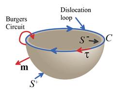
2. Introduce a bounded, simply connected surface S inside the solid (see the figure above)  Denote the edge of this surface by a curve C $–$ this curve will correspond to the dislocation line.   The direction of the line will be denoted by a unit vector $\tau$ tangent to the curve.  There are, of course, two possible choices for this direction. Either one can be used.   The normal to S will be denoted by a unit vector $m$, which must be chosen so that the curve C encircles m in a counterclockwise sense when traveling in direction $\tau$.

 

3. Create an imaginary cut on S, so that the two sides of the cut are free to move independently.  In the derivation below, the two sides of the cut will be denoted by $S^{+}$ and $S^{-}$, chosen so that the unit vector $m$ points from $S^{-}$ to $S^{+}$.

 

4. Hold $S^{+}$ fixed, displace $S^{-}$ by the burgers vector b, and weld the two sides of the cut back together.  Remove the constraint on $S^{+}$.

 

 

This procedure creates a displacement field that is consistent with the Burger’s circuit convention described in Section 5.3.4.  To see this, suppose that a crystal lattice is embedded within the elastic solid.  Perform a Burgers circuit around the curve C. Start the circuit on $S^{+}$, encircle the curve according to the right hand screw convention with respect to the line sense $\tau$, and end at $S^{-}$.   The end of the circuit is displaced by a distance b from the start, so that $b_i=u_i^{-}-u_i^{+}$.

 

The displacement and stress due to the dislocation loop can be calculated from

$\begin{array}{l}{u}_k(x)={\displaystyle \underset{S}{\int }{m}_i{\Sigma }_{ij}^{(k)}(x-\xi )b_{j}d{A}_{\xi }}\\ {\sigma }_{pq}(\xi )={\displaystyle \frac{E}{2(1+\nu )}{\displaystyle \underset{C}{\int }\left({\in }_{pij}{\Sigma }_{im}^{(q)}(x-\xi )+{\in }_{qij}{\Sigma }_{im}^{(p)}(x-\xi )+{\displaystyle \frac{2\nu {\delta }_{pq}}{1-2\nu }{\in }_{kij}{\Sigma }_{mi}^{(k)}(x-\xi )}\right)}{b}_m{\tau }_{j}d{s}_{\xi }}\end{array}$

where ${\Sigma }_{ij}^{(k)}$ is defined in Section 5.8.3, and ${\in }_{ijk}$ is the permutation symbol.  The symbols $d{A}_{\xi }$ $d{s}_{\xi }$ denotes that $\xi$ is varied when evaluating the surface or line integral.  These results are also often expressed in the more compact form

$\begin{array}{l}{u}_k(x)={\displaystyle \frac{1}{8\pi }{\displaystyle \underset{S}{\int }\left\{\left[m_k{b}_j{\displaystyle \frac{\partial }{\partial x_j}+m_j{b}_k{\displaystyle \frac{\partial }{\partial x_j}+{\displaystyle \frac{\nu b_j{m}_j}{1-\nu }{\displaystyle \frac{\partial }{\partial x_k}}}}}\right]{\displaystyle \frac{{\partial }^{2}R(x-\xi )}{\partial x_i\partial x_i}-{\displaystyle \frac{b_i{m}_j}{1-\nu }{\displaystyle \frac{{\partial }^{3}R(x-\xi )}{\partial x_i\partial x_j\partial x_k}}}}\right\}d{A}_{\xi }}}\\ {\sigma }_{pq}(x)={\displaystyle \frac{E}{16\pi (1+\nu )}{\displaystyle \underset{C}{\int }\left(\left[{\in }_{imp}{b}_m{\tau }_q+{\in }_{imq}{b}_m{\tau }_p\right]{\displaystyle \frac{{\partial }^{3}R(x-\xi )}{\partial x_i\partial x_j\partial x_j}}\right)}d{s}_{\xi }}\\ +{\displaystyle \frac{E}{8\pi (1-{\nu }^2)}{\displaystyle \underset{C}{\int }\left(b_m{\in }_{imk}{\tau }_k\left[{\displaystyle \frac{{\partial }^{3}R(x-\xi )}{\partial x_i\partial x_p\partial x_q}-{\delta }_{pq}{\displaystyle \frac{{\partial }^{3}R(x-\xi )}{\partial x_i\partial x_j\partial x_j}}}\right]\right)}d{s}_{\xi }}\end{array}$

where $R(x-\xi )=\sqrt{\left(x_k-{\xi }_k\right)\left(x_k-{\xi }_k\right)}$. 

 

 

Derivation:

 

1. Start with the reciprocal theorem

${\displaystyle \underset{S}{\int }{n}_i{\sigma }_{ij}^A{u}_j^{B}dA}+{\displaystyle \underset{V}{\int }{\rho }_0{b}_i^A{u}_i^{B}dV}={\displaystyle \underset{S}{\int }{n}_i{\sigma }_{ij}^B{u}_j^{A}dA}+{\displaystyle \underset{V}{\int }{\rho }_0{b}_i^B{u}_i^{A}dV}$

 

2. For state A, choose the actual stress and displacement in the solid containing the dislocation loop.   For state B, choose the stress, strain and displacement induced by a Dirac delta distribution of body force acting in the $e_k$ direction at position $\xi$ in the solid.  The displacements and stresses due to a Dirac delta distribution of body force are denoted by the functions $U_i^{(k)}(x)$ and ${\Sigma }_{ij}^{(k)}(x)$ defined in the preceding section.

 

3. When evaluating the reciprocal theorem, the two sides of the cut are treated as separate surfaces. Substituting into the reciprocal theorem and using the properties of the delta distribution gives

$\begin{array}{l}{\displaystyle \underset{S+}{\int }{n}_i^{+}{\sigma }_{ij}{U}_j^{(k)}(x-\xi )d{A}_x}+{\displaystyle \underset{S-}{\int }{n}_i^{-}{\sigma }_{ij}{U}_j^{(k)}(x-\xi )d{A}_x}\\ ={\displaystyle \underset{S+}{\int }{n}_i^{+}{\Sigma }_{ij}^{(k)}(x-\xi )u_j^{+}d{A}_x}+{\displaystyle \underset{S-}{\int }{n}_i^{-}{\Sigma }_{ij}^{(k)}(x-\xi )u_j^{-}d{A}_x}+u_i(\xi )\end{array}$

where $n^{+}=-m$ and $n^{-}=m$ denote the outward normals to the two sides of the cut, and $u_i^{\pm }$ denote the limiting values of the displacement field for the dislocation solution on the two sides of the cut.

 

4. Substituting for n, collecting together the surface integrals and noting that ${\sigma }_{ij}$ and $U_i^{(k)}(x)$ are continuous across S gives

$0={\displaystyle \underset{S}{\int }{m}_i{\Sigma }_{ij}^{(k)}(x-\xi )(u_j^{-}-u_j^{+})}d{A}_x+u_k(\xi )$

Finally, noting that $u_i^{-}-u_i^{+}=b_i$ (the burgers vector is the displacement of a material point at the end of the burgers circuit as seen from a point at the start) and that ${\Sigma }_{ij}^{(k)}(x-\xi )=-{\Sigma }_{ij}^{(k)}(\xi -x)$ yields the formula for displacements.

 

5. To calculate the stress, start by differentiating the displacement to see that

${\displaystyle \frac{\partial u_k}{\partial x_l}={\displaystyle \underset{S}{\int }{\displaystyle \frac{\partial }{\partial x_l}{m}_i{\Sigma }_{ij}^{(k)}(x-\xi )b_j}}d{A}_{\xi }}$

 

6. Next, observe that this can be expressed as an integral around the dislocation line

${\displaystyle \frac{\partial u_k}{\partial x_l}={\displaystyle \underset{C}{\int }{\in }_{lij}{\Sigma }_{im}^{(k)}(x-\xi )b_m}{\tau }_{j}d{A}_{\xi }}$

To see this, recall Stoke’s theorem, which states that

${\displaystyle \underset{S}{\int }{\in }_{npj}{\displaystyle \frac{\partial F_j}{\partial {\xi }_p}{m}_{n}d{A}_{\xi }={\displaystyle \underset{C}{\int }{F}_j{\tau }_{j}d{s}_{\xi }}}}$

for any differentiable vector field $F_j(\xi )$, integrated over a surface S with normal m that is bounded by curve C. Apply this to the line integral, use ${\in }_{npj}{\in }_{lij}={\delta }_{nl}{\delta }_{pi}-{\delta }_{ni}{\delta }_{pl}$, note that $\partial {\Sigma }_{im}^k/\partial {\xi }_i=0$ because $\Sigma$ is a static equilibrium stress field, and finally note that $\partial {\Sigma }_{ij}^{(k)}/\partial x_l=-\partial {\Sigma }_{ij}^{(k)}/\partial {\xi }_l$.

 

7. Finally, calculate the stress using the elastic stress-strain equation

${\sigma }_{pq}={\displaystyle \frac{E}{2(1+\nu )}\left({\delta }_{pk}{\delta }_{ql}+{\delta }_{qk}{\delta }_{pl}\right){\displaystyle \frac{\partial u_k}{\partial {\xi }_l}+{\displaystyle \frac{E\nu }{(1+\nu )(1-2\nu )}{\delta }_{pq}{\displaystyle \frac{\partial u_k}{\partial {\xi }_k}}}}}$

 

8. The alternative forms for the displacement and stress follow by noting that

$\begin{array}{l}{U}_i^{(k)}(x)={\displaystyle \frac{(1+\nu )}{4\pi E}\left\{{\delta }_{ik}{\displaystyle \frac{{\partial }^{2}R}{\partial x_j\partial x_j}-{\displaystyle \frac{1}{2(1-\nu )}{\displaystyle \frac{{\partial }^{2}R}{\partial x_i\partial x_k}}}}\right\}}\\ {\Sigma }_{ij}^{(k)}(x)={\displaystyle \frac{1}{8\pi }\left\{\left[{\delta }_{ik}{\displaystyle \frac{\partial }{\partial x_j}+{\delta }_{jk}{\displaystyle \frac{\partial }{\partial x_i}+{\displaystyle \frac{\nu {\delta }_{ij}}{1-\nu }{\displaystyle \frac{\partial }{\partial x_k}}}}}\right]{\displaystyle \frac{{\partial }^{2}R}{\partial x_n\partial x_n}-{\displaystyle \frac{1}{1-\nu }{\displaystyle \frac{{\partial }^{3}R}{\partial x_i\partial x_j\partial x_k}}}}\right\}}\end{array}$