5.9 Rayleigh-Ritz method for estimating natural frequency of an elastic solid

 

We conclude this chapter by describing an energy based method for estimating the natural frequency of vibration of an elastic solid.

 

 

 

5.9.1 Mode shapes and natural frequencies; orthogonality of mode shapes and Rayleighs Principle

 

It is helpful to review the definition of natural frequencies and mode shapes for a vibrating solid.  To this end, consider a representative elastic solid $–$ say a slender beam that is free at both ends, as illustrated below.

 

 

 The physical significance of the mode shapes and natural frequencies of the vibrating beam can be visualized as follows:

 

1. Suppose that the beam is made to vibrate by bending it into some (fixed) deformed shape $u_i=u_i^{(0)}(x_1,x_2,x_3)$; and then suddenly releasing it.   In general, the resulting motion of the beam will be very complicated, and may not even appear to be periodic.

 

2. However, there exists a set of special initial deflections $u_i^{(0)}=U_i^{(n)}(x_1,x_2,x_3)$, which cause every point on the beam to experience simple harmonic motion at some (angular) frequency ${\omega }_n$, so that the deflected shape has the form $u_i(x_k,t)=U_i^{(n)}(x_k)\cos {\omega }_{n}t$.

 

3. The special frequencies ${\omega }_n$ are called the natural frequencies of the system, and the special initial deflections $U_i^{(n)}(x_1,x_2,x_3)$ are called the mode shapes.  

 

4. A continuous system always has an infinite number of mode shapes and natural frequencies. The vibration frequencies and their modes are conventionally ordered as a sequence ${\omega }_1,{\omega }_2,{\omega }_3\mathrm{...}$ with ${\omega }_{n+1}>{\omega }_n$.  The lowest frequency of vibration is denoted ${\omega }_1$. The mode shapes for the lowest natural frequencies tend to have a long wavelength; the wavelength decreases for higher frequency modes.  If you are curious, the exact mode shapes and natural frequencies for a vibrating beam are derived in Section 10.4.1.

 

5. In practice the lowest natural frequency of the system is of particular interest, since design specifications often prescribe a minimum allowable limit for the lowest natural frequency.

 

 

We will derive two important results below, which give a quick way to estimate the lowest natural frequency.  Consider a linear elastic solid with elastic moduli $C_{ijkl}$ and mass density $\rho$, which occupies a volume V and has a surface S.   A part of the surface $S_2$ may be prevented from moving (or subjected to some time-independent displacement).   Let $U_i^{(n)}(x_1,x_2,x_3)$ be the displacements associated with the natural modes of vibration.  Then

 

1. The mode shapes are orthogonal, which means that the displacements associated with two different vibration modes $U_i^{(k)}$ and $U_i^{(j)}$ have the property that

${\displaystyle \underset{V}{\int }{U}_i^{(k)}(x_n)}{U}_i^{(j)}(x_n)dV=0(k\ne j)$

 

2. We will prove Rayleigh’s principle, which can be stated as follows.  Let ${\widehat{U}}_i(x_k)$ denote any kinematically admissible displacement field (you can think of this as a guess for the mode shape), which must be differentiable, and must satisfy ${\widehat{U}}_i(x_k)=0$ on $S_1$.  Define measures of potential energy $\widehat{V}$ and kinetic energy $\widehat{T}$ associated with ${\widehat{U}}_i(x_k)$ as

$\widehat{V}={\displaystyle \underset{V}{\int }{\displaystyle \frac{1}{2}{C}_{ijkl}{\displaystyle \frac{\partial {\widehat{U}}_k}{\partial x_l}}}}{\displaystyle \frac{\partial {\widehat{U}}_i}{\partial x_j}dV{\omega }^2\widehat{T}={\displaystyle \underset{V}{\int }{\displaystyle \frac{1}{2}\rho {\omega }^2{\widehat{U}}_i{\widehat{U}}_i}}dV}$

Then

${\displaystyle \frac{\widehat{V}}{\widehat{T}}\ge {\omega }_1^2,\text{and}{\displaystyle \frac{\widehat{V}}{\widehat{T}}={\omega }_1^2\text{if and only if}{\widehat{U}}_i=U_i^{(1)}}}$

The result is useful because the fundamental frequency can be estimated by approximating the mode shape in some convenient way, and minimizing $\widehat{V}/\widehat{T}$.

 

 

 

Orthogonality of mode shapes

 

We consider a generic linear elastic solid, with elastic constants $C_{ijkl}$ and mass density $\rho$. Note that

 

1. External forces do not influence the natural frequencies of a linear elastic solid, so we can assume that the body force acting on the interior of the solid is zero.

 

2. Part of the boundary $S_1$ may be subjected to prescribed displacements.  When estimating vibration frequencies, we can assume that the displacements are zero everywhere on $S_1$

 

3. The remainder of the boundary $S_2$ can be assumed to be traction free.

 

 

By definition the mode shapes and natural frequencies have the following properties:

 

1. The displacement field associated with this vibration mode is $u_i(x_k,t)=U_i^{(n)}(x_k)\cos {\omega }_{n}t$

 

2. The displacement field must satisfy the equation of motion for a linear elastic solid given in Section 5.1.2, which can be expressed in terms of the mode shape and natural frequency as

$C_{ijkl}{\displaystyle \frac{{\partial }^2{u}_k}{\partial x_i\partial x_l}=\rho {\displaystyle \frac{{\partial }^2{u}_j}{\partial t^2}\Rightarrow C_{ijkl}{\displaystyle \frac{{\partial }^2{U}_k^{(n)}}{\partial x_i\partial x_l}+\rho {\omega }_n^2{U}_j^{(n)}=0}}}$

 

3. The mode shapes must satisfy $U_i^{(n)}(x_k)=0$ on $S_1$ to meet the displacement boundary condition, and $C_{ijkl}\left(\partial U_k^{(n)}/\partial x_l\right)n_i=0$ on $S_2$ to satisfy the traction free boundary condition.

 

 

Orthogonality of the mode shapes can be seen as follows.

 

1. Let  $U_i^{(m)}$ and $U_i^{(n)}$ be two mode shapes, with corresponding vibration frequencies ${\omega }_m$  and ${\omega }_n$. Since both mode shapes satisfy the governing equations (item 2 above), it follows that

$\begin{array}{l}{\displaystyle \underset{V}{\int }\left(C_{ijkl}{\displaystyle \frac{{\partial }^2{U}_k^{(n)}}{\partial x_i\partial x_l}{U}_j^{(m)}+\rho {\omega }_n^2{U}_j^{(n)}{U}_j^{(m)}}\right)}dV=0\\ {\displaystyle \underset{V}{\int }\left(C_{ijkl}{\displaystyle \frac{{\partial }^2{U}_k^{(m)}}{\partial x_i\partial x_l}{U}_j^{(n)}+\rho {\omega }_m^2{U}_j^{(m)}{U}_j^{(n)}}\right)}dV=0\end{array}$

 

2. Next, we show that

${\displaystyle \underset{V}{\int }{C}_{ijkl}{\displaystyle \frac{{\partial }^2{U}_k^{(n)}}{\partial x_i\partial x_l}{U}_j^{(m)}dV}}={\displaystyle \underset{V}{\int }{C}_{ijkl}{\displaystyle \frac{{\partial }^2{U}_k^{(m)}}{\partial x_i\partial x_l}{U}_j^{(n)}}}dV$

To see this, integrate both sides of this expression by parts.  For example, for the left hand side,

$\begin{array}{l}{\displaystyle \underset{V}{\int }{C}_{ijkl}{\displaystyle \frac{{\partial }^2{U}_k^{(n)}}{\partial x_i\partial x_l}{U}_j^{(m)}dV}}={\displaystyle \underset{V}{\int }{\displaystyle \frac{\partial }{\partial x_i}\left(C_{ijkl}{\displaystyle \frac{\partial U_k^{(n)}}{\partial x_l}{U}_j^{(m)}}\right)}}dV-{\displaystyle \underset{V}{\int }{C}_{ijkl}{\displaystyle \frac{\partial U_k^{(n)}}{\partial x_l}{\displaystyle \frac{\partial U_j^{(n)}}{\partial x_i}dV}}}\\ ={\displaystyle \underset{S}{\int }\left(C_{ijkl}{\displaystyle \frac{\partial U_k^{(n)}}{\partial x_l}{U}_j^{(m)}}\right)n_{i}dA}-{\displaystyle \underset{V}{\int }{C}_{ijkl}{\displaystyle \frac{\partial U_k^{(n)}}{\partial x_l}{\displaystyle \frac{\partial U_j^{(m)}}{\partial x_i}dV}}}\\ =-{\displaystyle \underset{V}{\int }{C}_{ijkl}{\displaystyle \frac{\partial U_k^{(n)}}{\partial x_l}{\displaystyle \frac{\partial U_j^{(m)}}{\partial x_i}dV}}}\end{array}$

where we have used the divergence theorem, and noted that the integral over the surface of the solid is zero because of the boundary conditions for $U_i^{(m)}$ and $U_i^{(n)}$.  An exactly similar argument shows that

${\displaystyle \underset{V}{\int }{C}_{ijkl}{\displaystyle \frac{{\partial }^2{U}_k^{(m)}}{\partial x_i\partial x_l}{U}_j^{(n)}dV}}=-{\displaystyle \underset{V}{\int }{C}_{ijkl}{\displaystyle \frac{\partial U_k^{(m)}}{\partial x_l}{\displaystyle \frac{\partial U_j^{(n)}}{\partial x_i}dV}}}$

Recalling that $C_{ijkl}=C_{klij}$ shows the result.

 

3. Finally, orthogonality of the mode shapes follows by subtracting the second equation in (1) from the first, and using (2) to see that

$\left({\omega }_n^2-{\omega }_m^2\right){\displaystyle \underset{V}{\int }\left(U_j^{(n)}{U}_j^{(m)}\right)}dV=0$

If m and n are two distinct modes with different natural frequencies, the mode shapes must be orthogonal.

 

 

Proof of Rayleigh’s principle

 

1. Note first that any kinematically admissible displacement field can be expressed as a linear combination of mode shapes as

${\widehat{U}}_i={\displaystyle \sum _{n=1}^{\infty }{\alpha }_n{U}_i^{(n)}}{\alpha }_m={\displaystyle \frac{{\displaystyle \underset{V}{\int }{\widehat{U}}_i{U}_i^{(m)}dV}}{{\displaystyle \underset{V}{\int }{U}_i^{(m)}{U}_i^{(m)}dV}}}$

To see the formula for the coefficients ${\alpha }_m$, multiply both sides of the first equation by $U_i^{(m)}$, integrate over the volume of the solid, and use the orthogonality of the mode shapes.

 

2. Secondly, note that the mode shapes satisfy

${\displaystyle \underset{V}{\int }{C}_{ijkl}{\displaystyle \frac{\partial U_k^{(m)}}{\partial x_l}{\displaystyle \frac{\partial U_j^{(n)}}{\partial x_i}dV}}}=\left\{\begin{array}{c}{\omega }_m^2{\displaystyle \underset{V}{\int }\left(U_j^{(m)}{U}_j^{(m)}\right)}dVm=n\\ 0m\ne n\end{array}\right.$

To see this, note first that because $U_i^{(m)}$ satisfies the equation of motion, it follows that

${\displaystyle \underset{V}{\int }\left(C_{ijkl}{\displaystyle \frac{{\partial }^2{U}_k^{(m)}}{\partial x_i\partial x_l}{U}_j^{(m)}+\rho {\omega }_m^2{U}_j^{(m)}{U}_j^{(m)}}\right)}dV=0$

Next, integrate the first term in this integral by parts (see step (2) in the poof of orthogonality of the mode shapes), and use the orthogonality of the mode shapes to see the result stated.

 

3. We may now expand the potential and kinetic energy measures $\widehat{V}$ and $\widehat{T}$ in terms of sums of the mode shapes as follows

$\begin{array}{l}\widehat{V}={\displaystyle \underset{V}{\int }{\displaystyle \frac{1}{2}{C}_{ijkl}\left({\displaystyle \sum _{n=1}^{\infty }{\alpha }_n{\displaystyle \frac{\partial U_j^{(n)}}{\partial x_i}}}\right)}}\left({\displaystyle \sum _{m=1}^{\infty }{\alpha }_m{\displaystyle \frac{\partial U_k^{(m)}}{\partial x_l}}}\right)={\displaystyle \frac{1}{2}\rho {\displaystyle \sum _{m=1}^{\infty }{\omega }_m^2{\alpha }_m^2}{\displaystyle \underset{V}{\int }\left(U_j^{(m)}{U}_j^{(m)}\right)}dV}\\ \widehat{T}={\displaystyle \underset{V}{\int }{\displaystyle \frac{\rho }{2}\left({\displaystyle \sum _{n=1}^{\infty }{\alpha }_n{U}_j^{(n)}}\right)}}\left({\displaystyle \sum _{m=1}^{\infty }{\alpha }_m{U}_j^{(m)}}\right)dV={\displaystyle \frac{1}{2}\rho {\displaystyle \sum _{m=1}^{\infty }{\alpha }_m^2}{\displaystyle \underset{V}{\int }\left(U_j^{(m)}{U}_j^{(m)}\right)}}\end{array}$

where we have used the result given in step (2) and orthogonality of the mode shapes.

 

4. Finally, we know that ${\omega }_m\ge {\omega }_1$ for $m\ge 1$, which shows that

$\widehat{V}\ge {\displaystyle \frac{1}{2}\rho {\omega }_1^2{\displaystyle \sum _{m=1}^{\infty }{\alpha }_m^2}{\displaystyle \underset{V}{\int }\left(U_j^{(m)}{U}_j^{(m)}\right)}dV}$

We see immediately that $\widehat{V}/\widehat{T}\ge {\omega }_1^2$, with equality if and only if ${\alpha }_m=0$ for $m>1$

 

 

 

5.9.2 Estimate of natural frequency of vibration for a beam using Rayleigh-Ritz method

 

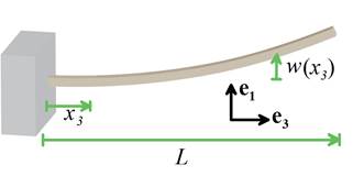
The figure below illustrates the problem to be solved: an initially straight beam has Young’s modulus $E$ and mass density $\rho$, and its cross-section has area A and moment of area $I$.  The left hand end of the beam is clamped, the right hand end is free.  We wish to estimate the lowest natural frequency of vibration.

 

 

The deformation of a beam can be characterized by the deflection $w(x)$ of its neutral section.  The potential energy of the beam can be calculated from the formula derived in Section 5.6.4, while the kinetic energy measure T can be approximated by assuming the entire cross-section displaces with the mid-plane without rotation, which gives

$V(w)={\displaystyle \underset{0}{\overset{L}{\int }}{\displaystyle \frac{1}{2}EI{\left\{{\displaystyle \frac{d^{2}w(x_3)}{d{x}_3{}^2}}\right\}}^{2}d{x}_3}}$    $T(w)={\displaystyle \underset{0}{\overset{L}{\int }}{\displaystyle \frac{1}{2}\rho A{\left\{w(x_3)\right\}}^{2}d{x}_3}}$

The natural frequency can be estimated by selecting a suitable approximation for the mode shape $\widehat{W}$, and minimizing the ratio $V/T$, as follows:

 

1. Note that the mode shape must satisfy the boundary conditions $\widehat{W}=d\widehat{W}/d{x}_1=0$.  We could try a polynomial $\widehat{W}=x_1^2+C{x}_1^3$, where C is a parameter that can be adjusted to get the best estimate for the natural frequency.

 

2. Substituting this estimate into the definitions of V and T and evaluating the integrals gives

${\displaystyle \frac{V}{T}={\displaystyle \frac{EI}{\rho A{L}^4}{\displaystyle \frac{420(1+3CL+3C^2{L}^2)}{(15C^2{L}^2+35CL+21)}}}}$

 

3. To get the best estimate for the natural frequency, we must minimize this expression with respect to C.  It is straightforward to show that the minimum value occurs for $CL=\left(\sqrt{39}-12\right)/15$. Substituting this value back into the results of step (2) gives

${\displaystyle \frac{V}{T}=12.48{\displaystyle \frac{EI}{\rho A{L}^4}\ge {\omega }^2}}$

 

4. For comparison, the formula for exact natural frequency of the lowest mode is derived in Section 10.4.1, and gives ${\omega }^2=12.36EI/(\rho A{L}^4)$.