9.2 Stress and strain based fracture and fatigue
criteria
Many of the most successful design
procedures use simple, experimentally calibrated, functions of stress and
strain to assess the likelihood of failure in a component. Some examples of commonly used failure
criteria are summarized in this section.
9.2.1 Stress based failure criteria for brittle solids
and composites.
Experiments show that brittle solids (such as ceramics,
glasses, and fiber-reinforced composites) tend to fail when the stress in the
solid reaches a critical magnitude.
Materials such as ceramics and glasses can be idealized using an isotropic failure criterion. Composite materials are stronger when loaded
in some directions than others, and must be modeled using an anisotropic failure criterion.
Failure criteria for isotropic
materials
The simplest brittle fracture
criterion states that fracture is initiated when the greatest tensile principal
stress in the solid reaches a critical magnitude
(The subscript TS stands for tensile strength). To apply the criterion, you must
1. Measure (or look up) for the material. can be measured by conducting tensile tests on
specimens it is important to test a large number of
specimens because the failure stress is likely to show a great deal of
statistical scatter. The tensile strength
can also be measured using beam bending tests.
The failure stress measured in a bending test is referred to as the
`modulus of rupture’ for the material. It is nominally equivalent to but in practice usually turns out to be
somewhat higher.
2. Calculate the anticipated stress
distribution in your component or structure (e.g. using FEM). Finally, you plot contours of principal
stress, and find the maximum value .
If the design is safe (but be sure to use an
appropriate factor of safety!).
Failure criteria for anisotropic
materials
More sophisticated criteria must be
used to model anisotropic materials (especially composites). The criteria must take account for the fact
that the material is stronger in some directions than others. For example, a fiber reinforced composite is
usually much stronger when loaded parallel to the fiber direction than when loaded
transverse to the fibers. There are many
different ways to account for this anisotropy a few approaches are summarized below.
 Orientation dependent fracture strength. One approach
is to make the tensile strength of the solid orientation dependent. For example, the tensile strength of a
brittle, orthotropic solid (with three distinct, mutually perpendicular
characteristic material directions) could be characterized by its tensile
strengths parallel to the three characteristic
directions in the solid.
The tensile strength when loaded
parallel to a general direction could be interpolated between these values as
Orientation dependent fracture strength. One approach
is to make the tensile strength of the solid orientation dependent. For example, the tensile strength of a
brittle, orthotropic solid (with three distinct, mutually perpendicular
characteristic material directions) could be characterized by its tensile
strengths parallel to the three characteristic
directions in the solid.
The tensile strength when loaded
parallel to a general direction could be interpolated between these values as
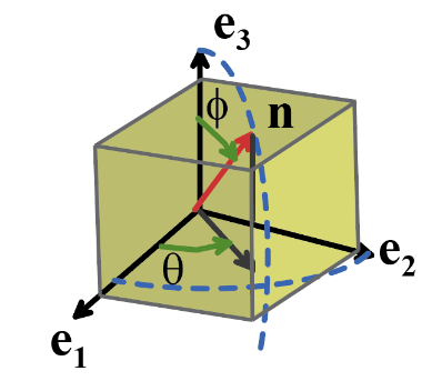
where are illustrated in the figure. The material
fails if the stress acting normal to any plane in the solid exceeds the
fracture stress for that plane, i.e.
where are the stress components in the basis .
To use this criterion to check for failure at any point in the solid,
you must
(i) Find the components of stress in
the basis;
(ii) Maximize the function with respect to ; and
(iii) Check whether the maximum value
of exceeds 1.
If so, the material will fail; if not, it is safe.
Goldenblat-Kopnov failure criterion. A very general phenomenological failure criterion can
be constructed by simply combining the stress components in a basis oriented
with respect to material axes as polynomial function. The Goldenblat-Kopnov
criterion is one example, which states that the critical stresses required to
cause failure satisfy the equation
Here A and B are material constants:
A is diagonal ( ) and has the same symmetries as the elasticity
tensor, i.e. .
The most general anisotropic material would therefore be characterized
by 24 independent material constants, but in practice simplified versions have
far fewer parameters. Most failure
criteria for composites are in fact special cases of the Goldenblat-Kopnov
criterion, including the Tsai-Hill criterion outlined below.
Tsai-Hill criterion: The Tsai-Hill criterion is used
to model damage in brittle laminated fiber-reinforced composites and wood. A
specimen of laminated composite subjected to in-plane loading is sketched below.
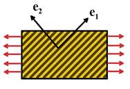
The Tsai-Hill criterion assumes that a plane
stress state exists in the solid. Let denote the nonzero components of stress, with
basis vectors and oriented parallel and perpendicular to the
fibers in the sheet, as shown. The
Tsai-Hill failure criterion is
at failure, where , and are material properties. They are measured as follows:
1. The laminate is loaded in uniaxial
tension parallel to the fibers. The material fails when
2. The laminate is loaded in uniaxial
tension perpendicular to the fibers. The
material fails when
3. In principle, the laminate could be
loaded in shear it would then fail when . In practice it is preferable to
pull on the laminate in uniaxial tension with stress at 45 degrees to the fibers, which induces
stress components .
A simple calculation then shows that .
9.2.2 Probabilistic Design Methods for Brittle
Fracture (Weibull Statistics)
The fracture criterion is too crude for many applications. The tensile strength of a brittle solid
usually shows considerable statistical scatter, because the likelihood of
failure is determined by the probability of finding a large flaw in a highly
stressed region of the material. This
makes it difficult to determine an unambiguous value for tensile strength should you use the median value of your
experimental data? Pick the stress level
where 95% of specimens survive? It’s better to deal with this problem using a
more rigorous statistical approach.
Weibull statistics refers to a
technique used to predict the probability of failure in a brittle
material. The following approach is used
1. Test a large number of samples with
identical size and shape under uniform tensile stress, and determine their
survival probability as a function of stress (survival probability is
approximated by the fraction of specimens that survive a given stress level).
2. 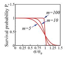 Fit the survival probability of these
specimens is fit by a Weibull distribution
Fit the survival probability of these
specimens is fit by a Weibull distribution
where and m are material constants. The distribution is illustrated on the right.
The index m is typically of
the order 5-10 for ceramics, and is independent of specimen volume. The parameter is the stress at which the probability of
survival is exp(-1), (about 37%). This critical stress depends on the specimen volume , and is smaller for larger
specimens.
3. Given m, and the corresponding specimen volume , the survival probability of a
volume of material subjected to uniform uniaxial
stress follows as
To see this, note that the volume V
can be thought of as containing specimens.
The probability that they all survive is .
4. More generally, the survival
probability of a solid subjected to an arbitrary stress distribution with
principal values can be computed as
where
This approach is quite successful in
some applications: for example, it explains why brittle materials appear to be
stronger in bending than in uniaxial tension.
Like many statistical approaches it has some limitations as a design
tool. The method can predict accurately
the stress that gives 30% probability of failure. But who wants to buy a product that has a 30%
probability of failure? For design
applications we need to predict the probability of 1 failure in a million or so. It is very difficult to measure the tail
of a statistical distribution accurately, and a distribution that was fit to
predict 63% failure probability may be wildly inaccurate in the region of
interest.
9.2.3 Static Fatigue Criterion for Brittle Materials
`Static fatigue’ refers to the
progressive reduction in tensile strength of a stressed brittle material with
time. The simplest way to model static
fatigue is to make the tensile strength of the material a function of time and
applied stress. The usual approach is to
set
where is the maximum principal stress acting on the
solid, which may vary slowly with time t;
is the tensile strength of the solid at time t=0, and are two material constants. Typically m
has values between 5 and 10. For the
particular case of a constant stress,
we see that
Since failure occurs when , the time to failure follows as
so that and m
can easily be determined by measuring the time to failure in uniaxial tension
as a function of applied stress.
Under
multi-axial loading, the maximum principal tensile stress should be used for .
9.2.4 Constitutive laws for crushing failure of
brittle materials
 Brittle materials are generally used
in applications where they are subjected primarily to compressive stress.
Brittle materials are very strong in compression, but they will fail if
subjected to combined hydrostatic compression and shear (e.g. by loading in
uniaxial compression). Failure in
compression is a consequence of distributed microcracking in the solid large numbers of small cracks nucleate,
propagate for a short while and then arrest.
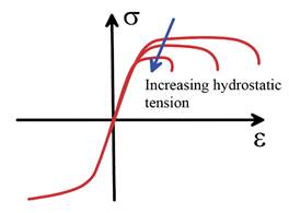
Failure occurs as a result of coalescence of these cracks. A typical stress-strain curve during compression
of a brittle material, such as concrete, is illustrated on the right. Failure
in compression is less catastrophic than tension, and in some respects
qualitatively resembles metal plasticity. For plastically deforming metals, however, the
stress-strain curve is independent of hydrostatic stress. In contrast, the crushing resistance of a
brittle material increases with hydrostatic compression.
Brittle materials are generally used
in applications where they are subjected primarily to compressive stress.
Brittle materials are very strong in compression, but they will fail if
subjected to combined hydrostatic compression and shear (e.g. by loading in
uniaxial compression). Failure in
compression is a consequence of distributed microcracking in the solid large numbers of small cracks nucleate,
propagate for a short while and then arrest.
Failure occurs as a result of coalescence of these cracks. A typical stress-strain curve during compression
of a brittle material, such as concrete, is illustrated on the right. Failure
in compression is less catastrophic than tension, and in some respects
qualitatively resembles metal plasticity. For plastically deforming metals, however, the
stress-strain curve is independent of hydrostatic stress. In contrast, the crushing resistance of a
brittle material increases with hydrostatic compression.
This type of crushing is often
modeled using constitutive equations based on small-strain metal plasticity. The governing equations for a simple,
small-strain, constitutive model of this form will be summarized briefly here. A
more detailed discussion of plasticity theory is given in Section 3.6.
The material is characterized by the
following properties:
· The Young’s modulus E and Poisson ratio
· The stress-v-plastic strain curve
measured from a uniaxial compression test, which is fit by a functional
relation of the form , where is the magnitude of the compressive
strain. Any of the functions listed in
Section 3.6.5 could be used for the function Y.
· A material constant c, which controls how rapidly the
strength of the material increases with hydrostatic compression.
The constitutive equations specify a relationship between an
increment in stress applied to the material and an increment in
strain , as follows
1. The strain is decomposed into elastic
and irreversible (damage) parts as
;
2. The elastic part of the strain is related
to the stress by the linear elastic constitutive equations
3. The critical stress that initiates
crushing damage is given by a failure criterion (analogous to the yield
criterion for a metal) of the form
where , , and is the accumulated irreversible strain. Notice
that the failure criterion depends on the hydrostatic part of the stress:
unlike yield in metals, the material becomes more resistant to fracture if p<0.
4. The plastic strain components are
determined using an associated flow rule
5. The magnitude of the plastic strain
increment is related to the stress increment by
where is the slope of the uniaxial stress-strain
curve, and for , while for .
HEALTH WARNING: These constitutive equations should only be used in regions where the
hydrostatic stress is compressive ( ). In
regions of hydrostatic tension, a tensile brittle fracture criterion should be
used for example, the material could be assumed to
lose all load bearing capacity if the principal tensile stress exceeds a
critical magnitude.
9.2.5 Ductile Fracture
Criteria
Strain to failure approach: Ductile fracture in tension occurs by
the nucleation, growth and coalescence of voids in the material. A crude criterion for ductile failure could
be based on the accumulated plastic strain, for example
at failure, where is the plastic strain to failure in a uniaxial
tensile test.
 Porous metal plasticity: Experiments show that the strain to
cause ductile failure in a material depends on the hydrostatic component of
tensile stress acting on the specimen, as shown on the right. For example, the strain to failure under
torsional loading (which subjects the material to shear with no hydrostatic
stress) is much greater than under uniaxial tension. The critical strain is
influenced by hydrostatic stress because ductile failure occurs as a result of
the nucleation and growth of cavities in the solid. A hydrostatic stress greatly increases the
rate of growth of the cavities. The simple strain-to-failure approach cannot
account for this behavior.
Porous metal plasticity: Experiments show that the strain to
cause ductile failure in a material depends on the hydrostatic component of
tensile stress acting on the specimen, as shown on the right. For example, the strain to failure under
torsional loading (which subjects the material to shear with no hydrostatic
stress) is much greater than under uniaxial tension. The critical strain is
influenced by hydrostatic stress because ductile failure occurs as a result of
the nucleation and growth of cavities in the solid. A hydrostatic stress greatly increases the
rate of growth of the cavities. The simple strain-to-failure approach cannot
account for this behavior.
Porous metal plasticity was developed
to address this issue. The basic idea is
simple: the solid is idealized as a plastic matrix which contains a volume
fraction of cavities.
To model the solid, the plastic stress-strain laws outlined in Sections 3.6
and 3.7 are extended to calculate the volume fraction of voids in the material
as part of the solution, and also to account for the weakening effect of the
voids. Failure is modeled by
constructing the plastic stress-strain law so that the material loses all its
strength at a critical void volume fraction.
Both rate independent and
viscoplastic versions of porous plasticity exist. The viscoplastic models have some advantages
for finite element computations, because the rate dependence can stabilize the
effects of strain softening. A simple
small-strain viscoplastic constitutive law with power-law hardening and
power-law rate dependence will be outlined here to illustrate the main features
of these models. The constitutive law is
known as the ‘Gurson model.’
The material is characterized by the
following properties:
· The Young’s modulus E and Poisson ratio ;
· A characteristic stress Y, a characteristic strain and strain hardening exponent n, which govern the strain hardening behavior of the matrix
material;
· A characteristic strain rate and strain rate exponent m, which govern the strain rate sensitivity of the solid;
· A constant , which controls the rate of void
nucleation with plastic straining;
· The flow strength of the matrix , the void volume fraction, , and the total accumulated effective
plastic strain in the matrix material which all evolve with plastic straining.
The constitutive equations specify a relationship between the
stress applied to the material and the resulting
strain rate , as follows
1. The strain rate is decomposed into
elastic and plastic parts as ;
2. The elastic part of the strain rate is
related to the stress rate by the linear elastic constitutive equations
3. The magnitude of the plastic strain rate is determined
by the following plastic flow potential
where , and .
Note that for the plastic strain rate increases with
hydrostatic stress p.
4. The components of the plastic strain
rate tensor are computed from an associated flow law
5. Strain hardening in the matrix is
modeled by relating its flow stress to the accumulated strain in the matrix . The following power-law hardening
model is often used
6. The effective plastic strain in the
matrix is calculated from the condition that the plastic dissipation in the
matrix must equal the rate of work done by stresses, which requires that
7. Finally, the model is completed by
specifying the void volume fraction as a function of strain. The void volume fraction can increase because
of growth of existing voids, or nucleation of new ones. To account for both
effects, one can set
where the first term
accounts for void growth, and the second accounts for strain controlled void
nucleation.
LeMaitre Damage
Model The Gurson failure model is
appealing because it is based on a description of microscopic processes that
cause failure in a ductile metal. It
performs best when modeling materials that are subjected to a high value of
stress triaxiality (where is the von-Mises equivalent stress). Under these conditions voids remain close to
sphearical. For , voids tend to
elongate rather than grow, and the Gurson model is not accurate. The ‘LeMaitre’ damage model (LeMaitre, 1985)
and its many extensions were developed to address this problem.
The LeMaitre model
idealizes a ductile metal as an elastic-plastic matrix that contains a dilute
distribution of voids. At time t=0, the voids are spherical and have a
volume fraction . As the material is deformed the voids may
increase their volume; and may also elongate to become ellipsoids. Their shape is quantified by the ‘elongation
ratio’ (the ratio of the longest to the shortest
semi-axis of the ellipsoid. Since the
voids are initially spherical, it follows that at time t=0.
The matrix can be
characterized by any standard plasticity model: for example, it is often
assumed to be an elastic-plastic solid with power-law rate dependence and
power-law hardening. The matrix is
weakened by the voids, so (assuming small strains) the elastic and plastic
strain rates are related to the stresses by
where is the von-Mises effective stress; is the
von-Mises effective plastic strain, which evolves according to , and , are the elastic moduli and plastic properties
of the fully dense matrix material, respectively. Notice that, unlike the Gurson model, the
volumetric plastic strain rate is neglected in the LeMaitre formulation. This makes the model somewhat easier to implement
in a finite element code.
The voids grow and
change their shape as the material deforms.
Finite element simulations of an elastic-plastic material containing a
periodic array of cavities suggest that the rates of change of void volume
fraction and elongation ratio are given approximately by
where is the stress triaxiality, and are two functions that can be fit to finite
element simulations. For a power-law
hardening and rate dependent matrix they have the approximate form
The coefficients and the exponent depend on the properties of the matrix
material, but as a rough guide , , and .
Finally, the
material fails when the void volume fraction or elongation ratio reach critical
values or (whichever occurs first), where and are material properties that must be
determined by experiment.
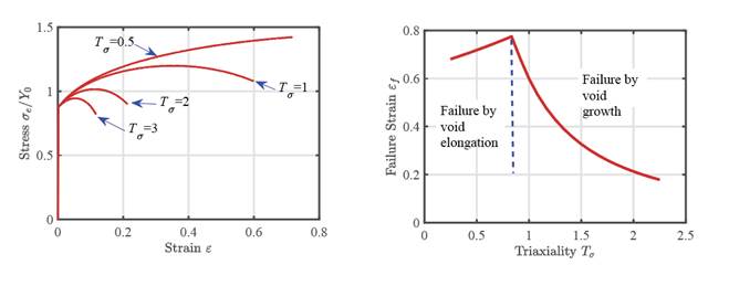
Some predictions of
the LeMaitre model are shown above. The
left hand figure shows the variation of normalized uniaxial stress with strain,
for several values of stress triaxiality . Material properties used in these
predictions are listed in the figure caption.
The material fails at the end of each stress-strain curve. The curves have to be interpreted rather
carefully: although they are uniaxial stress-strain curves, they are not what
would be measured if the stress-v-strain behavior were calculated from the load-v-displacement
response of a standard uniaxial tensile specimen. In practice, a tensile specimen will start
to neck at a strain significantly lower than that required to cause material
failure (a method for calculating the necking strain is described in Section
9.2.6). Necking causes the load to drop
and the plastic strain to localize in a small length of the specimen, which
causes the apparent stress and failure stress deduced from the tensile test to
be lower than the actual stress and strain in the material. The right hand figure shows the effective
strain at failure as a function of stress triaxiality. For failure occurs when , while for higher
triaxiality failure occurs when .
Johnson-Cook Damage
model. This is an example of a curve-fit to failure
data, which does not attempt to model the underlying mechanisms in detail. It is designed to predict failure at high
rates of strain, and is often used in simulations of machining, metal forming,
and impacts. Many modifications to the
original model can be found in the literature, which differ in the various
functions used to model strain hardening, rate dependence, and thermal
softening. Here, we outline a typical
example.
The Johnson-Cook
model is a modified elastic-visoplastic constitutive equation, in which damave
begins at a critical strain that depends on how the material is loaded, and the
flow stress decreases as the material is damaged, eventually dropping to zero. .
Damage is quantified by a two scalar variables, and . The first variable is used to predict the critical point at which
the material starts to lose its strength, with representing the initial, intact material, and
signifying that further straining will cause a
loss of strength (the subscript ‘N’ stands for ‘nucleation’). The second variable quantifies the loss of strength after damage
starts, with representing intact material and representing complete loss of strength. Since the model is intended to be used at
high strain rates, it also accounts for the effects of high temperatures that
may be generated during rapid plastic deformation. Accordingly, the plastic strain rate is
related to the stress by
where is the von-Mises effective stress; is the
von-Mises effective plastic strain, which evolves according to , and are material properties (these constants are
not independent, so can be assigned any convenient value before
the remaining parameters are fit to experiment). The function reduces the flow stress if the temperature T exceeds a ‘softening temperature’ , to a value of zero
at the melting temperature . Thus
The damage nucleation parameter evolves with
plastic strain as
where
is the plastic
strain at the start of damage nucleation in a material element subjected to a
constant strain rate and stress triaxiality.
The coefficients are material properties that must be fit to
experimental data. The strength
parameter evolves as
where with is the plastic strain at at the point of
complete loss of strength, in a material element that is subjected to a
constant strain rate and stress triaxiality.
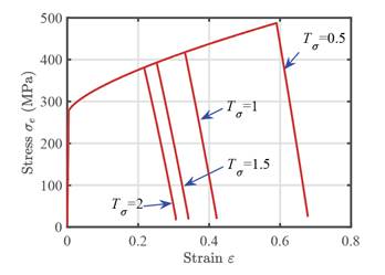
The figure below shows representative stress-strain
curves predicted by the Johnson-Cook model, using material properties (listed
in the figure caption) that represent an Aluminum alloy. The stress-strain curve is independent of
stress triaxiality until damage begins. Beyond the damage nucleation strain,
the stress drops to zero along an approximately straight-line curve with steep
(negative) slope. Failure occurs at
lower strains for higher stress triaxiality.
General guidelines
for using damage models: The models listed
here, along with many other similar damage models are all designed to be used
in finite element simulations. They
need to be used with caution, however.
The following points may help guide their use:
1. The models are useful as a way to compare
the failure resistance of different designs.
For this purpose it is not necessary to use very accurate values for
material parameters, and while the critical conditions necessary to cause
failure may not be predicted precisely, the qualitative effects of making
changes to the geometry of the design are usually predicted correctly.
2. All models assume that damage decreases the
strength of the material. The uniaxial
stress-strain curve usually has at least a small portion with negative slope,
so the material is not Drucker stable in this portion. This usually results in strain localization
(plastic strain is concentrated in a narrow region such as a neck or shear
band) and finite element predictions are generally strongly sensitive to mesh
size after the onset of localization, and may not converge to a well defined
limit even as the mesh size is reduced towards zero. Many commercial code use some ad-hoc
procedures to reduce the mesh sensitivity, but these are not based on any
rigorous theory, and predictions with different codes may differ.
3. It is possible to find values for material
properties for the damage models listed here in the literature, for most
materials of practical interest. The
properties are very sensitive to the microstructure and composition of the
materials, however, so literature values are unlikely to be a good fit to a
particular material you may be interested in.
For accurate predictions, you will need to measure the properties of
your material.
4. It is difficult to measure the material
properties that govern failure.
Designing specimens that deform the material under a state of constant
stress triaxiality is particularly difficult.
Both high and low triaxiality is difficult to achieve under controlled
conditions. A standard tensile specimen has a stress triaxiality of only 1/3
(prior to necking). Notched round bars
can increase the maximum triaxiality in the specimen to between 0.5 and 1, but
the stress state in these specimens is non-uniform. At the opposite extreme, it is difficult to
subject a material to a large shear strain at a constant low stress
triaxiality, because deformation in the gage section tends to change the stress
state. In addition, a large number of
tests are usually required to ensure statistically meaningful data, and the
tests need to be repeated any time a change is made to the material’s
microstructure and composition. Even
different heats of a steel can have significantly different properties. Most organizations that rely on computational
simulations to model failure (e.g. crash or forming simulations) have
proprietary procedures for calibrating their models. These have been refined
over many years to give designers confidence in their predictions.
5. Finally, the predictions of damage models
are reliable only if the stress and strain histories during service loading are
similar to those in the laboratory specimens that were used to measure the
properties of the material. Most lab
tests are designed to subject material to proportional loading (i.e. the
principal stress and strain directions are fixed). The damage models described here will not be
reliable for non-proportional or cyclic loading.
9.2.6 Ductile failure by strain localization
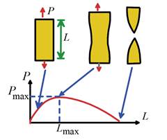 If you test a cylindrical specimen of
a very ductile material in uniaxial tension, it will initially deform uniformly,
and remain cylindrical. At a critical load (or strain) the specimen will start
to neck, as shown on the right. Necking, once it starts, is usually unstable there is a concentration in stress near the
necked region, increasing the rate of plastic flow near the neck compared with
the rest of the specimen, and so increasing the rate of neck formation. The strains in the necked region rapidly
become very large, and quickly lead to failure.
If you test a cylindrical specimen of
a very ductile material in uniaxial tension, it will initially deform uniformly,
and remain cylindrical. At a critical load (or strain) the specimen will start
to neck, as shown on the right. Necking, once it starts, is usually unstable there is a concentration in stress near the
necked region, increasing the rate of plastic flow near the neck compared with
the rest of the specimen, and so increasing the rate of neck formation. The strains in the necked region rapidly
become very large, and quickly lead to failure.
Neck formation is a consequence of geometric
softening. A very simple model
explains the concept of geometric softening.
1. Consider a cylindrical specimen with
initial cross sectional area and length . The
specimen is subjected to a load P, which deforms the material
plastically. After straining, the length of the specimen increases to L,
and its cross-sectional area decreases to A.
2. Assume that the material is perfectly
plastic and has a true stress-strain curve (Cauchy stress v- logarithmic strain) that can be
approximated by a power-law with n<1.
3. The true strain in the specimen is
related to its length by
4. The force on the specimen is related
to the Cauchy stress by
5. At the point of maximum load
6. We can calculate by noting that the volume of the specimen is
constant during plastic straining, which shows that
Notice that is negative this means that the specimen tends to soften
as a result of the change in its cross sectional area. This is what is meant by geometric softening.
7. We can calculate from (2) and (3) as follows
Notice that is positive strain hardening in the material tends to
compensate for the effects of geometric softening.
8. Finally, substituting the results of
(6) and (7) back into (5) and recalling that
shows that at the point of maximum load, the
strain and length of the specimen are
9. Finally, note that by volume
conservation the cross sectional area is , so the maximum load the specimen
can withstand follows as
It turns out that the point of
maximum load coincides with the condition for unstable neck formation in the
bar. This is plausible a falling load displacement curve is always a
sign that there might be a possibility of non-unique solutions but a rather sophisticated calculation is
required to show this rigorously.
There are two important points to take away from this
discussion.
· Plastic localization, as opposed to
material failure, may limit load bearing capacity;
· If you measure the strain to failure
of a material in uniaxial tension, it is possible that you have not measured
the inherent strength of the material your specimen may have failed because of a
geometric effect. Material behavior does
influence the strain to failure, of course: the simple analysis of geometric
softening shows that the strain hardening behavior of the material is
critical. Material damage and geometric
instability are often closely coupled, with damage causing some initial
softening in the material that then causes the instability; which in turn
intensifies the plastic strain and further damage.
Plastic localization can occur for
many reasons. There are two general
classes of localization it may occur as a consequence of changes in
specimen geometry (i.e. geometric softening); or it may occur due to a natural
tendency of the material itself to soften at large strains.
Examples of geometry induced
localization are
1. Neck formation in a bar under uniaxial
tension;
2. Localized thinning in a sheet metal
as it is stretched by a die;
3. Shear band formation in torsional or
shear loading at high strain rate due to thermal softening as a result of
plastic heat generation
Examples of material induced localization are
1. Localization in a Gurson solid due to
the softening effect of voids at large strains;
2. Localization in a single crystal due
to the softening effect of lattice rotations;
3. Localization in a brittle
microcracking material due to the increase in elastic compliance caused by the
cracks.
Geometric localization can be modeled
quite easily, because it does not rely on any empirical failure criteria. A straightforward FEM computation, with an
appropriate constitutive law and proper consideration of finite strains, will
predict localization if it is going to occur the only thing you need to worry about is to
be sure you understand what triggered the localization. Localization can start at a geometric
imperfection in the model, in which case your prediction is meaningful (but may
be sensitive to the nature of the imperfection). It may also be triggered by numerical errors,
in which case the predicted failure load is meaningless. It is usually exceedingly difficult to
compute what happens after localization, because predictions with
standard plasticity models are strongly mesh dependent, and in some cases do
not converge as the mesh is refined.
Fortunately, it’s not often necessary to do this when designing a part.
There are also some situations where
it is impossible to use a finite element mesh that is fine enough to resolve
the geometric instability. One such
example is a finite element simulation of sheet metal stamping. The sheet is often modeled using shell
elements, which cannot resolve the complex 3D stress and strain states that
develop around a neck. In this
situation, necking is treated as a material failure, which assumed to occur
when some combination of the principal strains in the sheet (or sometimes the
principal stresses) reach a critical value. The failure condition is often
quantified by a ‘forming limit diagram,’ illustrated below.
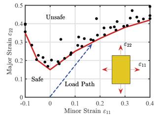
The points on the graph show the
experimentally measured strain to failure in a sheet that was subjected to biaxial
stretching at a (nominally) constant ratio of the two principal strain rates .
These tests are usually performed by stretching the material using a
die, with a specially shaped workpiece that achieves the desired strain path
(the two standard tests are called the ‘Marciniak’ and ‘Nakajima’ tests). A curve is then drawn under the data points
to show the range of strains that the sheet can tolerate without failure. The curve is then used as a failure
criterion. This sounds
straightforward, but in practice it can be very difficult to determine the
critical strain at failure accurately. It is important to follow any applicable
standards to achieve repeatable results.
Simulations also have to be done carefully, because predictions can be
very sensitive to mesh size.
Organizations that rely on these procedures often have proprietary
protocols for calibrating the forming limit diagrams and simulating the forming
process. These are developed over long
experience and are changed only with great care.
9.2.7 Criteria for failure by high cycle
fatigue under constant amplitude cyclic loading
Empirical stress or strain based life prediction methods are
extensively used in design applications.
The approach is straightforward subject a sample of the material to a cycle of
stress (or strain) that resembles service loading, in an environment
representative of service conditions, and measure its life as a function of
stress (or strain) amplitude, then fit the data with a curve.
Here we will review criteria that are
used to predict fatigue life under proportional cyclic loading. A typical
stress cycle is parameterized by its amplitude and the mean stress , as shown below.
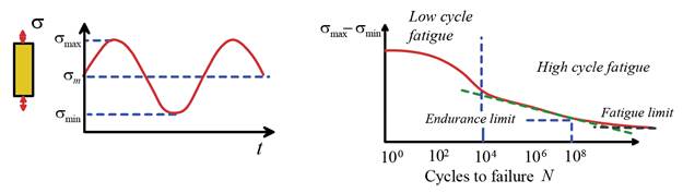
For tests run in the high cycle
fatigue regime with any fixed value of mean stress, the relationship
between stress amplitude and the number of cycles to failure N
is fit well by Basquin’s Law
where the exponent b is typically between 0.05 and
0.15. The constant C is a
function of mean stress.
There are two ways to account for the
effects of mean stress. Both are based
on the same idea: we know that if the mean stress is equal to the tensile
strength of the material , it will fail in 0 cycles of
loading. We also know that for zero mean
stress, the fatigue life obeys Basquin’s law.
We can interpolate between these two points. There are two ways to do this:
· Goodman’s rule uses a linear
interpolation, giving
where is the constant in Basquin’s law determined by
testing at zero mean stress.
· Gerber’s rule uses a parabolic fit
In practice, experimental data seem
to lie between these two limits.
Goodman’s rule gives a safe estimate.
These criteria are intended to be
used for components that are subjected to uniaxial tensile stress. The criteria can still be used if the loading
is proportional (i.e. with fixed
directions of principal stress). In this
case, the maximum principal stress should be used to calculate and .
They do not work under non-proportional loading. A very large number of fatigue models have
been developed for more general loading conditions a review can be found in Liu
and Mahadevan, (2005).
9.2.8 Criteria for failure by low cycle
fatigue
If a fatigue test is run with a high
stress level (sufficient to cause plastic flow in a large section of the solid)
the specimen fails very quickly (less than 10 000 cycles). This regime of behavior is known as `low
cycle fatigue’. The fatigue life
correlates best with the plastic strain amplitude rather than stress amplitude,
and it is found that the Coffin Manson Law
gives a good fit to empirical data (the constants C
and b do not have the same values as for Basquin’s law, of course)
9.2.9 Criteria for failure under
variable amplitude cyclic loading
 Fatigue tests are usually done at constant
stress (or strain) amplitude. Service
loading usually involves cycles with variable (and often random)
amplitude. Fortunately, there’s a
remarkably simple way to estimate fatigue life under variable loading using
constant stress data.
Fatigue tests are usually done at constant
stress (or strain) amplitude. Service
loading usually involves cycles with variable (and often random)
amplitude. Fortunately, there’s a
remarkably simple way to estimate fatigue life under variable loading using
constant stress data.
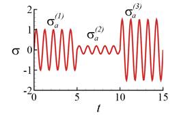
Suppose the load history is comprised
of a set of load cycles at a stress amplitude , followed by a set of cycles at load amplitude and so on (see the figure on the right). For the ith set of cycles at load
amplitude , we could compute the number of
cycles that would cause the specimen to fail using Basquin’s law
The Miner-Palmgren failure criterion assumes a linear summation
of damage as a result of each set of load cycles, so that at failure
In terms of stress amplitude
The same approach works under low cycle fatigue conditions,
in which case
 The criterion is often used under
random loading. A typical random stress history is illustrated on the right. To apply Miner’s rule, we need to find a way
to estimate the number of cycles of load at a given stress level. There are various ways to do this one approach is to count the peaks in the load
history, and compute the probability of finding a peak at stress level . (Of course, this only works if the
signal has well defined peaks - this is not the case for white noise, for
example).
The criterion is often used under
random loading. A typical random stress history is illustrated on the right. To apply Miner’s rule, we need to find a way
to estimate the number of cycles of load at a given stress level. There are various ways to do this one approach is to count the peaks in the load
history, and compute the probability of finding a peak at stress level . (Of course, this only works if the
signal has well defined peaks - this is not the case for white noise, for
example).
Miner’s rule then predicts that the number of cycles to
failure satisfies
