9.5 Plastic fracture mechanics

 

Thus far we have avoided discussing the complicated material behavior in the process zone near the crack tip.  This is acceptable as long as the process zone is small compared with the specimen dimensions, and a clear zone of K dominance is established around the crack tip.  In some structures, however, the materials are so tough and ductile that the plastic zone near the crack tip is huge $–$ and comparable to specimen dimensions.  Linear elastic fracture mechanics cannot be used under these conditions.  Instead, we adopt a framework based on plastic solutions to crack tip fields. 

 

In this section, we address three issues:

 

1. The size of the plastic zone at the crack tip is estimated

 

2. The asymptotic fields near the crack tip in a plastic material are calculated

 

3. A phenomenological framework for predicting fracture in plastic solids is outlined.

 

 

 

9.5.1 Dugdale-Barenblatt cohesive zone model of yield at a crack tip

 

The simplest estimate of the size of the plastic zone at a crack tip can be obtained using Dugdale & Barenblatt’s cohesive zone model, which gives the plastic zone size at the tip of a crack in a thin sheet (deforming under conditions of plane stress) as

$r_p\approx {\displaystyle \frac{\pi }{8}{\left({\displaystyle \frac{K_I}{Y}}\right)}^2}$

where $K_I$ is the crack tip stress intensity factor and Y is the material yield stress. 

 

This estimate is derived as follows.  Consider a crack of length 2a in an elastic-perfectly plastic material with elastic constants $E,\nu$ and yield stress Y.  We assume that the specimen is a thin sheet, with thickness much less than crack length, so that a state of plane stress is developed in the solid.  We anticipate that there will be a region near each crack tip where the material deforms plastically.  The Mises equivalent stress $\sqrt{3S_{ij}{S}_{ij}/2}$ should not exceed yield in this region.   It’s hard to find a solution with stresses at yield everywhere in the plastic zone, but we can easily construct an approximate solution where the stress along the line of the crack satisfies the yield condition, using the ‘cohesive zone’ model illustrated in below

 

 

 

Let $r_p$ denote the length of the cohesive zone at each crack tip.  To construct an appropriate solution we extend the crack in both directions to put fictitious crack tips at $x_1=\pm \left(a+r_p\right)$, and distribute tractions of magnitude $Y$ over the crack flanks from $x_1=a$ to $x_1=a+r_p$, and similarly at the other crack tip..  Evidently, the stress then satisfies ${\sigma }_{22}=Y$ along the line of the crack just ahead of each crack.  

 

We can use point force solution given in the table in Section 9.3.3 to compute the stress intensity factor at the fictitious crack tip. Omitting the tedious details of evaluating the integral, we find that

$K_I^{*}=\left(\sigma -Y\right)\sqrt{\pi (a+r_p)}+{\displaystyle \frac{2Y}{\pi }\sqrt{\pi (a+r_p)}{\sin }^{-1}{\displaystyle \frac{a}{a+r_p}}}$

The * on the stress intensity factor is introduced to emphasize that this is not the true crack tip stress intensity factor (which is of course $K_I=\sigma \sqrt{\pi a}$ ), but the stress intensity factor at the fictitious crack tip. The stresses must remain bounded just ahead of the fictitious crack tip, so that $r_p$ must be chosen to satisfy $K_I^{*}=0$.  This gives

$r_p={\displaystyle \frac{a}{\sin \left(\pi [1-\sigma /Y]/2\right)}-a\approx {\displaystyle \frac{{\pi }^2}{8}{\left({\displaystyle \frac{\sigma }{Y}}\right)}^{2}a}}$

Its more sensible to express this in terms of stress intensity factor

$r_p\approx {\displaystyle \frac{\pi }{8}{\left({\displaystyle \frac{K_I}{Y}}\right)}^2}$

This estimate turns out to be remarkably accurate for plane stress conditions, where more detailed calculations give

$r_p={\displaystyle \frac{1}{\pi }{\left({\displaystyle \frac{K_{IC}}{Y}}\right)}^2}$

For plane strain the plastic zone is smaller: detailed calculations show that the plastic zone size is

$r_p={\displaystyle \frac{1}{3\pi }{\left({\displaystyle \frac{K_{IC}}{Y}}\right)}^2}$

 

 

 

9.5.2 Hutchinson-Rice-Rosengren (HRR) crack tip fields for stationary crack in a power law hardening solid

 

The HRR fields are an exact solution to the stress, strain and displacement fields near a crack tip in a power-law strain hardening, rigid plastic material, which is subjected to monotonically increasing stress at infinity.  The model is based on the following assumptions:

 

1. The solid is infinitely large, and contains an infinitely long crack with its tip at the origin;

 

2. The material is a rigid plastic, strain hardening solid with uniaxial stress -v- strain curve

$\sigma ={\sigma }_0{(\epsilon /{\epsilon }_0)}^{1/n}$

where ${\sigma }_0,{\epsilon }_0,n$ are material properties, with n>1.

 

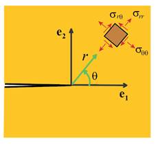The HRR solution shows that the stress, strain and displacement fields at a point $(r,\theta )$ in the solid (see the figure)  can be calculated from functions of the form

$\begin{array}{l}{\sigma }_{ij}={\sigma }_0{\left({\displaystyle \frac{J}{{\sigma }_0{\epsilon }_{0}r}}\right)}^{1/(n+1)}{\Sigma }_{ij}(\theta ,n)\\ {\epsilon }_{ij}={\epsilon }_0{\left({\displaystyle \frac{J}{{\sigma }_0{\epsilon }_{0}r}}\right)}^{n/(n+1)}{E}_{ij}(\theta ,n)\\ u_i={\displaystyle \frac{J}{{\sigma }_0}{\left({\displaystyle \frac{{\sigma }_0{\epsilon }_{0}r}{J}}\right)}^{1/(n+1)}{U}_i(\theta ,n)}\end{array}$

where ${\Sigma }_{ij},E_{ij},U_i$ are dimensionless functions of the angle $\theta$ and the hardening index n only, and J is the value of the (path independent) J integral

$J={\displaystyle \underset{C}{\int }(W({\sigma }_e){\delta }_{j1}-{\sigma }_{ij}{\displaystyle \frac{\partial u{}_i}{\partial x_1})m_{j}ds}}$

where

$W={\displaystyle \frac{n}{n+1}{\sigma }_0{\epsilon }_0{\left({\displaystyle \frac{3S_{ij}{S}_{ij}}{2{\sigma }_0}}\right)}^{n+1}}$

with $S_{ij}={\sigma }_{ij}-{\sigma }_{kk}{\delta }_{ij}/3$.  W can be interpreted as the total work done in loading the material up to a stress ${\sigma }_{ij}$ under monotonically increasing, proportional loading.

 

These results are important for two reasons:

 

1. They show that the magnitudes of the stress, strain and displacement near the crack tip are characterized by J.  Thus, in highly plastic materials, J can replace K as the fracture criterion.

 

2. They illustrate the nature of the stress and strain fields near the crack tip.  In particular, they show that the stress has a $r^{-(n+1)}$ singularity $–$ for n=1 (a linear stress-strain curve) we recover the square root singularity found in elastic materials; while for a perfectly plastic solid ( $n\to \infty$ ) the stress is constant.  In contrast, the strains have a square root singularity for n=1 and an $r^{-1}$ singularity for $n\to \infty$

 

 

Derivation  The HRR solution is derived by solving the following governing equations for displacements $u_i$, strains ${\epsilon }_{ij}$ and stresses ${\sigma }_{ij}$ 

 

· Strain-displacement relation ${\epsilon }_{ij}=(\partial u_i/\partial x_j+\partial u_j/\partial x_i)/2$

 

· Stress equilibrium $\partial {\sigma }_{ij}/\partial x{}_i=0$

 

· Boundary conditions ${\sigma }_{22}={\sigma }_{12}=0$ on $x_2=0x_1<0$

 

· The stress-strain relation for a power-law hardening rigid plastic material subjected to monotonically increasing, proportional loading (this means that material particles are subjected to stresses and strains whose principal axes don’t rotate during loading) can be expressed as

${\epsilon }_{ij}={\epsilon }_0{\left({\displaystyle \frac{{\sigma }_e}{{\sigma }_0}}\right)}^n{\displaystyle \frac{3}{2}{\displaystyle \frac{S_{ij}}{{\sigma }_e}{S}_{ij}={\sigma }_0{\left({\displaystyle \frac{{\epsilon }_e}{{\epsilon }_0}}\right)}^{1/n}{\displaystyle \frac{2}{3}{\displaystyle \frac{{\epsilon }_{ij}}{{\epsilon }_0}}}}}$

where ${\epsilon }_0,{\sigma }_0,n$ are material constants and $S_{ij}={\sigma }_{ij}-{\sigma }_{kk}{\delta }_{ij}/3$ is the deviatoric stress and ${\sigma }_e=\sqrt{3S_{ij}{S}_{ij}/2}$ is the Von Mises effective stress.  Of course, we don’t know a priori that material elements ahead of a crack tip experience proportional loading, but this can be verified after the solution has been found.  It is helpful to note that under proportional loading, the rigid plastic material is indistinguishable from an elastic material with strain energy potential

$W={\displaystyle \frac{n}{n+1}{\sigma }_0{\epsilon }_0{\left({\displaystyle \frac{{\sigma }_e}{{\sigma }_0}}\right)}^{n+1}={\displaystyle \frac{n}{n+1}{\sigma }_0{\epsilon }_0{\left({\displaystyle \frac{{\epsilon }_e}{{\epsilon }_0}}\right)}^{(1+n)/n}}}$

The J integral must then be path independent.

 

 

The equilibrium condition may be satisfied through an Airy stress function $\varphi$, generating stresses in the usual way as

${\sigma }_{rr}={\displaystyle \frac{1}{r}{\displaystyle \frac{\partial \varphi }{\partial r}+{\displaystyle \frac{1}{r^2}{\displaystyle \frac{{\partial }^2\varphi }{\partial {\theta }^2}{\sigma }_{\theta \theta }={\displaystyle \frac{{\partial }^2\varphi }{\partial r^2}{\sigma }_{r\theta }=-{\displaystyle \frac{\partial }{\partial r}\left({\displaystyle \frac{1}{r}{\displaystyle \frac{\partial \varphi }{\partial \theta }}}\right)}}}}}}$

The solution can be derived from an Airy function that has a separable form

$\varphi =r^{\alpha }f\left(\theta \right)+\mathrm{...}$

where the power $\alpha$ and $f\left(\theta \right)$ are to be determined.

 

The strength of the singularity $\alpha$ can be determined using the J integral. Evaluating the integral around a circular contour radius r enclosing the crack tip we obtain

$J={\displaystyle \underset{C}{\int }(W{\delta }_{j1}-{\sigma }_{ij}{\displaystyle \frac{\partial u_i}{\partial x_1})m_{j}ds}}={\displaystyle \underset{-\pi }{\overset{\pi }{\int }}(W{\delta }_{j1}-{\sigma }_{ij}{\displaystyle \frac{\partial u_i}{\partial x_1})m_{j}rd\theta }}$

For the J integral to be path independent, it must be independent of r and therefore W must be of order $r^{-1}$.  The Airy function gives stresses of order $r^{\alpha -2}$, and the corresponding strain energy density would have order $r^{(n+1)(\alpha -2)}$.  Consequently, for a path independent J, we must have $(n+1)(\alpha -2)=-1$, so

$\alpha ={\displaystyle \frac{2n+1}{n+1}}$

Note for a linear material (n=1), we find $\alpha =3/2$, which corresponds to the expected square-root stress singularity.

 

We can now scale the governing equations as discussed in Section 7.2.13.   To this end, define normalized length, displacement, strain, stress and Airy function as

$X_i={\sigma }_0{\epsilon }_0{x}_i/JR={\sigma }_0{\epsilon }_{0}r/J{U}_i=u_i{\sigma }_0/J$

$E_{ij}=\epsilon {}_{ij}/{\epsilon }_0{\Sigma }_{ij}={\sigma }_{ij}/{\sigma }_0\Phi =\varphi {\left({\sigma }_0{\epsilon }_0/J\right)}^2$

With these definitions the governing equations reduce to

 

· Strain-displacement relation $E_{ij}=(\partial U_i/\partial X_j+\partial U_j/\partial X_i)/2$

 

· Stress equilibrium $\partial {\Sigma }_{ij}/\partial X{}_i=0$

 

· Constitutive equation

$E_{ij}={\left({\Sigma }_e\right)}^n{\displaystyle \frac{3}{2}{\displaystyle \frac{{{\Sigma }^{\prime }}_{ij}}{{\Sigma }_e}{{\Sigma }^{\prime }}_{ij}={\Sigma }_{ij}-{\Sigma }_{kk}{\delta }_{ij}/3{\Sigma }_e=\sqrt{3{\Sigma }_{ij}{\Sigma }_{ij}/2}}}$

 

In addition, the stresses are related to the normalized Airy function by

${\Sigma }_{rr}={\displaystyle \frac{1}{R}{\displaystyle \frac{\partial \Phi }{\partial R}+{\displaystyle \frac{1}{R^2}{\displaystyle \frac{{\partial }^2\Phi }{\partial {\theta }^2}{\Sigma }_{\theta \theta }={\displaystyle \frac{{\partial }^2\Phi }{\partial R^2}{\Sigma }_{r\theta }=-{\displaystyle \frac{\partial }{\partial R}\left({\displaystyle \frac{1}{R}{\displaystyle \frac{\partial \Phi }{\partial \theta }}}\right)}}}}}}$

while the expression for the J integral becomes

$1={\displaystyle \underset{-\pi }{\overset{\pi }{\int }}(\widehat{W}{\delta }_{j1}-{\Sigma }_{ij}{\displaystyle \frac{\partial U_i}{\partial X_1})m_{j}Rd\theta }}$

where $\widehat{W}=W/{\sigma }_0{\epsilon }_0$.  The only material parameter appearing in the scaled equations is n.  In addition, note that J has been eliminated from the equations, so the solution is independent of J.

 

The stresses can be derived from an Airy function

$\Phi =R^{(2n+1)/(n+1)}f(\theta )$

The scaling of displacements, strain and stress with load and material properties then follows directly from the definition of the normalized quantities. 

 

To compute the full expression for $f(\theta )$ and hence to determine ${\Sigma }_{ij},E_{ij},U_i$ is a tedious and not especially straightforward exercise.  The governing equation for $f$ is obtained from the condition that the strain field must be compatible.  This requires

$r^{-1}{\displaystyle \frac{\partial {\epsilon }_{rr}}{\partial r}-r^{-2}{\displaystyle \frac{{\partial }^2{\epsilon }_{rr}}{\partial {\theta }^2}-2r^{-1}{\displaystyle \frac{\partial {\epsilon }_{\theta \theta }}{\partial r}-{\displaystyle \frac{{\partial }^2{\epsilon }_{\theta \theta }}{\partial r^2}+r^{-1}{\displaystyle \frac{{\partial }^2{\epsilon }_{r\theta }}{\partial r\partial \theta }+r^{-2}{\displaystyle \frac{\partial {\epsilon }_{r\theta }}{\partial \theta }=0}}}}}}$

Computing the stresses from the Airy function, deducing the strains using the constitutive law and substituting the results into this equation yields a fourth order nonlinear ODE for f, which must be solved subject to appropriate symmetry and boundary conditions.  The solution must be found numerically $–$ details are given in Hutchinson (1968) and Rice and Rosengren (1968).

 

 

 

9.5.3. Plastic fracture mechanics based on J

 

There are many situations (e.g. in design of pressure vessels, pipelines, etc) where the structure is purposely made from a tough, ductile material. Usually, one cannot apply LEFM to these structures, because a large plastic zone forms at the crack tip (the plastic zone is comparable to specimen dimensions, and there is no K dominant zone).  Some other approach is needed to design against fracture in these applications.

 

Two related approaches are used $–$ one is based on the HRR crack tip field and uses J as a fracture criterion; the other uses the crack tip opening displacements as a fracture criterion.  Only the J based approach will be discussed here.

 

The most important conclusion from the HRR crack tip field is that the amplitude of stresses, strains and displacements near a crack tip in a plastically deforming solid scale in a predictable way with J.  Just as stress intensity factors quantify the stress and strain magnitudes in a linear elastic solid, J can be used as a parameter to quantify the state of stress near the tip of a crack in a plastic solid.

 

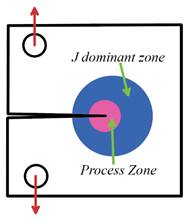Phenomenological J based fracture mechanics is based on the same reasoning that is used to justify K based LEFM.  We postulate that we will find three distinct regions in a plastically deforming specimen containing a crack (see the figure), namely

 

1. A process zone near the crack tip, with finite deformations and extensive material damge, where the asymptotic HRR field is not accurate

 

2. A J dominant zone, which is outside the process zone, but small compared with specimen dimensions. Here, the HRR field accurately describes the deformation

 

3. The remainder, where stress and strain fields are controlled by specimen geometry and loading.

 

 

As for LEFM, we hope that the process zone is controlled by the surrounding J dominant zone, so that crack tip loading conditions can be characterized by J.

 

J based fracture mechanics is applied in much the same way as LEFM.  We assume that crack growth starts when J reaches a critical value (for mode I plane strain loading this value is denoted $J_{IC}$ ).  The critical value must be measured experimentally for a given material, using standard test specimens.  To assess the safety of a structure or component containing a crack, one must calculate J and compare the predicted value to $J_{IC}$ - if $J<J_{IC}$ the structure is safe.

 

 

Practical application of J based fracture mechanics is somewhat more involved than LEFM.  Tests to measure  $J_{IC}$ are performed using standard test specimens $–$ deeply cracked 3 or 4 point bend bars are often used.  For example, calibrations for a 3 point bend bar shown below are available in J. R. Rice, P. C. Paris and J. G. Merkle (1973).

 

Calculating J for a specimen or component usually requires a full field FEM analysis.  Cataloging solutions to standard problems is much more difficult than for LEFM, because the results depend on the stress-strain behavior of the material.  Specifically, for a power-law solid containing a crack of length a and subjected to stress $\sigma$, we expect that

$J={\sigma }_0{\epsilon }_{0}a{(\sigma /{\sigma }_0)}^{n+1}f(n,geometry)$

For example, a slit crack of length 2a subjected to mode I loading with stress $\sigma$ has (approximately $–$ see He & Hutchinson (1981)

$J={\sigma }_0{\epsilon }_{0}a\pi \sqrt{n}{\left({\displaystyle \frac{\sqrt{3}\sigma }{{\sigma }_0}}\right)}^{n+1}$

Finally, to apply the theory it is necessary to ensure that both test specimen and component satisfy conditions necessary for J dominance.  As a rough rule of thumb, if all characteristic specimen dimensions (crack length, etc) exceed $200J/{\epsilon }_0{\sigma }_0$ J dominance is likely to be satisfied.