
Problems for Chapter 7
Introduction to Finite Element Analysis in Solid Mechanics
NOTE: The problems in the following section require a commercial finite element program. The problems have been tested using the commercial version of ABAQUS/CAE Ver 6.6 (available from http://www.simulia.com).
7.1. A guide to using commercial FE software
7.1.1. Please answer the following questions
7.1.1.1. What is the difference between a static and a dynamic FEA computation (please limit your answer to a sentence!)
7.1.1.2. What is the difference between the displacement fields in 8 noded and 20 noded hexahedral elements?
7.1.1.3. What is the key difference between the nodes on a beam element and the nodes on a 3D solid element?
7.1.1.4. Which of the boundary conditions shown below properly constrain the solid for a plane strain static analysis?


7.1.1.5. List three ways that loads can be applied to a finite element mesh
7.1.1.6. In a quasi-static analysis of a ceramic cutting tool machining steel, which surface would you choose as the master surface, and which would you choose as the slave surface?
7.1.1.7. Give three reasons why a nonlinear static finite element analysis might not converge.
7.1.2. You conduct an FEA computation to calculate the natural frequency of vibration of a beam that is pinned at both ends. You enter as parameters the Young’s modulus of the beam E, its area moment of inertia I, its mass per unit length m and its length L. Work through the dimensional analysis to identify a dimensionless functional relationship between the natural frequency and other parameters.
7.1.3. Please answer the FEA related questions
7.1.3.1. What is the difference between a truss element and a solid element (please limit your answer to a sentence!)
7.1.3.2. What is the difference between the displacement fields in 6 noded and 3 noded triangular elements, and which are generally more accurate?
7.1.3.3. Which of the boundary conditions shown below properly constrain the solid for a static analysis?


(a) (b) (c)
7.1.3.4. A linear elastic FE calculation predicts a maximum Mises stress of 100MPa in a component. The solid is loaded only by prescribing tractions and displacements on its boundary. If the applied loads and prescribed displacements are all doubled, what will be the magnitude of the maximum Mises stress?
7.1.3.5. An FE calculation is conducted on a part. The solid is idealized as an elastic-perfectly plastic solid, with Youngs modulus 210 GPa, Poisson ratio . Its plastic properties are idealized with Mises yield surface with yield stress 500MPa. The solid is loaded only by prescribing tractions and displacements on its boundary. The analysis predicts a maximum von-Mises stress of 400MPa in the component. If the applied loads and prescribed displacements are all doubled, what will be the magnitude of the maximum Mises stress?
|
|

7.1.4. The objective of this problem is to investigate the influence of element size on the FEA predictions of stresses near a stress concentration.
Set up a finite element model of the 2D (plane strain) part shown below (select the 2D button when creating the part, and make the little rounded radius by creating a fillet radius. Enter a radius of 2cm for the fillet radius). Use SI units in the computation (DO NOT USE cm!)
Use a linear elastic constitutive equation with . For boundary conditions, use zero horizontal displacement on AB, zero vertical displacement on AD, and apply a uniform horizontal displacement of 0.01cm on CD. Run a quasi-static computation.
Run computations with the following meshes:
7.1.4.1. Linear quadrilateral elements, with a mesh size 0.05 m
7.1.4.2. Linear quadrilateral elements, with mesh size 0.01 m
7.1.4.3. Linear quadrilateral elements with mesh size 0.005 m
7.1.4.4. Linear quadrilateral elements with a mesh size of 0.00125 m (this will have around 100000 elements and may take some time to run)
7.1.4.5. 8 noded (quadratic) quadrilateral elements with mesh size 0.005 m.
7.1.4.6. 8 noded (quadratic) quadrilateral with mesh size 0.0025 m.
For each mesh, calculate the maximum von Mises stress in the solid (you can just do a contour plot of Mises stress and read off the maximum contour value to do this). Display your results in a table showing the max. stress, element type and mesh size.
Clearly, proper mesh design is critical to get accurate numbers out of FEA computations. As a rough rule of thumb the element size near a geometric feature should be about 1/5 of the characteristic dimension associated with the feature in this case the radius of the fillet. If there were a sharp corner instead of a fillet radius, you would find that the stresses go on increasing indefinitely as the mesh size is reduced (the stresses are theoretically infinite at a sharp corner in an elastic solid)
|
|

7.1.5. In this problem, you will run a series of tests to compare the performance of various types of element, and investigate the influence of mesh design on the accuracy of a finite element computation.
We will begin by comparing the behavior of different element types. We will obtain a series of finite element solutions to the problem shown below. A beam of length L and with square cross section is subjected to a uniform distribution of pressure on its top face.
First, recall the beam theory solution to this problem. The vertical deflection of the neutral axis of the beam is given by
Here, is the load per unit length acting on the beam, and is the area moment of inertia of the beam about its neutral axis. Substituting and simplifying, we see that the deflection of the neutral axis at the tip of the beam is
Observe that this is independent of b, the thickness of the beam. A thick beam should behave the same way as a thin beam. In fact, we can take , in which case we should approach a state of plane stress. We can therefore use this solution as a test case for both plane stress elements, and also plane strain elements.

7.1.5.1. First, compare the predictions of beam theory with a finite element solution. Set up a plane stress analysis, with L=1.6m, h=5cm, E=210GPa, and p=100 . Constrain both and at the left hand end of the beam. Generate a mesh of plane stress, 8 noded (quadratic) square elements, with a mesh size of 1cm. Compare the FEM prediction with the beam theory result. You should find excellent agreement.
7.1.5.2. Note that beam theory does not give an exact solution to the cantilever beam problem. It is a clever approximate solution, which is valid only for long slender beams. We will check to see where beam theory starts to break down next. Repeat the FEM calculation for L=0.8, L=0.4, L=0.3, L=0.2, L=0.15, L=0.1. Keep all the remaining parameters fixed, including the mesh size. Plot a graph of the ratio of the FEM deflection to beam theory deflection as a function of L.
You should find that as the beam gets shorter, beam theory underestimates the deflection. This is because of shear deformation in the beam, which is ignored by simple Euler-Bernoulli beam theory (there is a more complex theory, called Timoshenko beam theory, which works better for short beams. For very short beams, there is no accurate approximate theory).
7.1.5.3. Now, we will use our beam problem to compare the performance of various other types of element. Generate a plane stress mesh for a beam with L=0.8m, h=5cm, E=210GPa, , p=100 , but this time use 4 noded linear elements instead of quadratic 8 noded elements. Keep the mesh size at 0.01m, as before. Compare the tip deflection predicted by FEA with the beam theory result. You should find that the solution is significantly less accurate. This is a general trend quadratic elements give better results than linear elements, but are slightly more expensive in computer time.
|
|
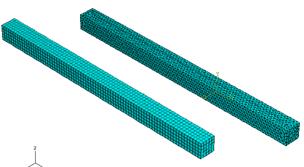
7.1.5.4. Run a similar test to investigate the performance of 3D elements. Generate the 3D meshes shown above, using both 4 and 8 noded hexahedral elements, and 4 and 10 noded tetrahedral elements. (Don’t attempt to model 2 beams together as shown in the picture; do the computations one at a time otherwise they will take forever).
Prepare a table showing tip deflection for 4 and 8 noded plane stress elements, 8 and 20 noded hexahedral elements, and 4 and 10 noded tetrahedral elements.
Your table should show that quadratic, square elements generally give the best performance. Tetrahedra (and triangles, which we haven’t tried … feel free to do so if you like…) generally give the worst performance. Unfortunately tetrahedral and triangular elements are much easier to generate automatically than hexahedral elements.
7.1.6. We will continue our comparison of element types. Set up the beam problem again with L=1.6m, h=5cm, E=210GPa, , p=100 , but this time use the plane strain mesh shown in the figure.
![]()
There are 16 elements along the length of the beam and 5 through the thickness. Generate a mesh with fully integrated 4 noded elements.
|
|

You should find that the results are highly inaccurate. Similar problems occur in 3d computations if the elements are severely distorted you can check this out too if you like.
This is due to a phenomenon know as `shear locking:’ the elements interpolation functions are unable to approximate the displacement field in the beam accurately, and are therefore too stiff. To understand this, visualize the deformation of a material element in pure bending. To approximate the deformation correctly, the sides of the finite elements need to curve, but linear elements cannot do this. Instead, they are distorted as shown. The material near the corners of the element is distorted in shear, so large shear stresses are generated in these regions. These large, incorrect, internal forces make the elements appear too stiff.
|
|

There are several ways to avoid this problem. One approach is to use a special type of element, known as a `reduced integration’ element. Recall that the finite element program samples stresses at each integration point within an element during its computation. Usually, these points are located near the corners of the elements. In reduced integration elements, fewer integration points are used, and they are located nearer to the center of the element (for a plane stress 4 noded quadrilateral, a single integration point, located at the element center, is used, as shown). There is no shear deformation near the center of the element, so the state of stress is interpreted correctly.
7.1.6.1. To test the performance of these reduced integration elements, change the element type in your computation to 4 noded linear quadrilaterals, with reduced integration. You should find much better results, although the linear elements are now a little too flexible.
7.1.6.2. Your finite element code may also contain more sophisticated element formulations designed to circumvent shear locking. `Incompatible mode’ elements are one example. In these elements, the shape functions are modified to better approximate the bending mode of deformation. If your finite element code has these elements, try them, and compare the finite element solution to the exact solution.
|
|
|
|


7.1.7. This problem demonstrates a second type of element locking, known as ‘Volumetric locking’. To produce it, set up the boundary value problem illustrated in the figures. Model only one quarter of the plate, applying symmetry boundary conditions as illustrated in the mesh. Assign an elastic material to the plate, with , E=210GPa, . Run the following tests:
7.1.7.1. Run the problem with fully integrated 8 noded plane strain quadrilaterals, and plot contours of horizontal, vertical and Von-Mises equivalent stress.
7.1.7.2. Modify to increase Poisson’s ratio to 0.4999 (recall that this makes the elastic material almost incompressible, like a rubber). horizontal, vertical and Von-Mises equivalent stress.. You should find that the mises stress contours look OK, but the horizontal and vertical stresses have weird fluctuations. This is an error the solution should be independent of Poisson’s ratio, so all the contours should look the way they did in part 1.
The error you observed in part 2 is due to volumetric locking. Suppose that an incompressible finite element is subjected to hydrostatic compression. Because the element is incompressible, this loading causes no change in shape. Consequently, the hydrostatic component of stress is independent of the nodal displacements, and cannot be computed. If a material is nearly incompressible, then the hydrostatic component of stress is only weakly dependent on displacements, and is difficult to compute accurately. The shear stresses (Mises stress) can be computed without difficulty. This is why the horizontal and vertical stresses in the example were incorrect, but the Mises stress was computed correctly. You can use two approaches to avoid volumetric locking.
7.1.7.3. Use `reduced integration’ elements for nearly incompressible materials. Switch the element type to reduced integration 8 noded quads, set Poisson’s ratio to 0.4999 and plot contours of horizontal, vertical and Mises stress. Everything should be fine.
7.1.7.4. You can also use a special `Hybrid element,’ which computes the hydrostatic stress independently. For fully incompressible materials, you must always use hybrid elements reduced integration elements will not work. Run the problem with hybrid elements using a Poisson’s 0.4999, and plot the same stress contours. As before, everything should work perfectly.
Clearly, elements must be selected with care to ensure accurate finite element computations. You should consider the following guidelines for element selection:
· Avoid using 3 noded triangular elements and 4 noded tetrahedral elements, except for filling in regions that may be difficult to mesh.
· 6 noded triangular elements and 10 noded tetrahedral elements are acceptable, but quadrilateral and brick elements give better performance.
· Fully integrated 4 noded quadrilateral elements and 8 noded bricks are usually specially coded to avoid volumetric locking, but are susceptible to shear locking. They can be used for most problems, although quadratic elements generally give a more accurate solution for the same amount of computer time.
· Use quadratic, reduced integration elements for general analysis work, except for problems involving large strains or complex contact.
· Use quadratic, fully integrated elements in regions where stress concentrations exist. Elements of this type give the best resolution of stress gradients.
· Use a fine mesh of linear, reduced integration elements or hybrid elements for simulations with very large strains.
7.1.8. A bar of material with square cross section with base 0.05m and length 0.2m is made from an isotropic, linear elastic solid with Young’s Modulus 207 GPa and Poisson’s ratio 0.3. Set up your commercial finite element software to compute the deformation of the bar, and use it to plot one or more stress-strain curves that can be compared with the exact solution. Apply a cycle of loading that first loads the solid in tension, then unloads to zero, then loads in compression, and finally unloads to zero again.
7.1.9. Repeat problem 7, but this time model the constitutive response of the bar as an elastic-plastic solid. Use elastic properties listed in problem7, and for plastic properties enter the following data
Plastic Strain |
Stress/MPa |
|
0 |
100 |
|
0.1 |
150 |
|
0.5 |
175 |
Subject the bar to a cycle of axial displacement that will cause it to yield in both tension and compression (subjecting one end to a displacement of +/-0.075m should work). Plot the predicted uniaxial stress-strain curve for the material. Run the following tests:
7.1.9.1. A small strain computation using an isotropically hardening solid with Von-Mises yield surface
7.1.9.2. A large strain analysis using an isotropically hardening solid with Von-Mises yield surface.
7.1.9.3. A small strain computation using a kinematically hardening solid
7.1.9.4. A large strain analysis with kinematic hardening
|
|

7.1.10. Use your commercial software to set up a model of a 2D truss shown in the figure. Make each member of the truss 2m long, with a steel cross section. Give the forces a 1000N magnitude. Mesh the structure using truss elements, and run a static, small-strain computation
Use the simulation to compute the elastic stress in all the members. Compare the FEA solution with the analytical result.
7.1.11. This problem has several objectives: (i) To demonstrate FEA analysis with contact; (ii) To illustrate nonlinear solution procedures and (iii) to demonstrate the effects of convergence problems that frequently arise in nonlinear static FEA analysis.
|
|

Set up commercial software to solve the 2D (plane strain) contact problem illustrated in the figure. Use the following procedure
- Create the part ABCD as a 2D deformable solid with a homogeneous section. Make the solid symmetrical about the axis
- Create the cylindrical indenter as a 2D rigid analytical solid. Make the cylinder symmetrical about the axis
- Make the block an elastic solid with
- Make the rigid surface just touch the block at the start of the analysis.
- Set the properties of the contact between the rigid surface and the block to specify a `hard,’ frictionless contact.
- To set up boundary conditions, (i) Set the vertical displacement of AB to zero; (ii) Set the horizontal displacement of point A to zero; and (iii) Set the horizontal displacement and rotation of the reference point on the cylinder to zero, and assign a vertical displacement of -2cm to the reference point.
- Create a mesh with a mesh size of 1cm with plane strain quadrilateral reduced integration elements.
7.1.11.1. Begin by running the computation with a perfectly elastic analysis this should run very quickly. Plot a graph of the force applied to the indenter as a function of its displacement.
7.1.11.2. Next, try an elastic-plastic analysis with a solid with yield stress 800MPa. This will run much more slowly. You will see that the nonlinear solution iterations constantly fail to converge as a result, your code should automatically reduce the time step to a very small value. It will probably take somewhere between 50 and 100 increments to complete the analysis.
7.1.11.3. Try the computation one more time with a yield stress of 500MPa. This time the computation will only converge for a very small time-step: the analysis will take at least 150 increments or so.
|
|

7.1.12. Set up your commercial finite element software to conduct an explicit dynamic calculation of the impact of two identical spheres, as shown below.
Use the following parameters:
- Sphere radius 2 cm
- Mass density 1000
- Young’s modulus , Poisson ratio
- First, run an analysis with perfectly elastic spheres. Then repeat the calculation for elastic-plastic spheres, with yield stress , , and again with
- Contact formulation hard contact, with no friction
- Give one sphere an initial velocity of =100m/s towards the other sphere.
Estimate a suitable time period for the analysis and step size based on the wave speed.
Finally, please answer the following questions:
7.1.12.1. Suppose that the main objective of the analysis is to compute the restitution coefficient of the spheres, defined as where denote the initial and final velocities of sphere A, and the same convention is used for sphere B. List all the material and geometric parameters that appear in the problem.
7.1.12.2. Express the functional relationship governing the restitution coefficient in dimensionless form. Show that for a perfectly elastic material, the restitution coefficient must be a function of a single dimensionless group. Interpret this group physically (hint - it is the ratio of two velocities). For an elastic-plastic material, you should find that the restitution coefficient is a function of two groups.
7.1.12.3. If the sphere radius is doubled, what happens to the restitution coefficient? (DON’T DO ANY FEA TO ANSWER THIS!)
7.1.12.4. Show that the kinetic energy lost during impact can be expressed in dimensionless form as
Note that the second term is very small for any practical application (including our simulation), so in interpreting data we need only to focus on behavior in the limit .
7.1.12.5. Use your plots of KE as a function of time to determine the change in KE for each analysis case. Hence, plot a graph showing as a function of
7.1.12.6. What is the critical value of where no energy is lost? (you may find it helpful to plot against log( ) to see this more clearly). If no energy is lost, the impact is perfectly elastic.
7.1.12.7. Hence, calculate the critical impact velocity for a perfectly elastic collision between two spheres of (a) Alumina; (b) Hardened steel; (c) Aluminum alloy and (d) lead
7.1.12.8. The usual assumption in classical mechanics is that restitution coefficient is a material property. Comment briefly on this assumption in light of your simulation results.