6.3 Bounding theorems in plasticity and their applications

 

To set the background for plastic limit analysis, it is helpful to review the behavior of an elastic-plastic solid or structure subjected to mechanical loading.  The solution to an internally-pressurized elastic-perfectly plastic sphere given in Section 6.1 provides a representative example.  All elastic-perfectly plastic structures will exhibit similar behavior.  In particular

 

· An inelastic solid will reach yield at some critical value of applied load.

 

· If the load exceeds yield, a plastic region starts to spread through the solid. As an increasing area of the solid reaches yield, the displacements in the structure progressively increase.

 

· At a critical load, the plastic region becomes large enough to allow unconstrained plastic flow in the solid. The load cannot be increased beyond this point. The solid is said to collapse. 

 

 

Strain hardening will influence the results quantitatively, but if the solid has a limiting yield stress (a stress beyond which it can never harden) its behavior will be qualitatively similar.

 

In a plasticity calculation, often the two most interesting results are (a) the critical load where the solid starts to yield; and (b) the critical load where it collapses.  Of course, we don’t need to solve a plasticity problem to find the yield point $–$ we only need the elastic fields.  In many design problems this is all we need, since plastic flow must be avoided more often than not.  But there are situations where some plasticity can be tolerated in a structure or component; and there are even some situations where it’s desirable (e.g. in designing crumple zones in cars).  In this situation, we usually would like to know the collapse load for the solid.  It would be really nice to find some way to get the collapse load without having to solve the full boundary value problem.

 

This is the motivation for plastic limit analysis.  The limit theorems of plasticity provide a quick way to estimate collapse loads, without needing any fancy calculations.  In fact, collapse loads are often much easier to find than the yield point!

 

In this section, we derive several useful theorems of plastic limit analysis and illustrate their applications.

 

 

 

6.3.1 Definition of the plastic dissipation

 

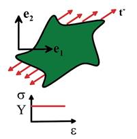
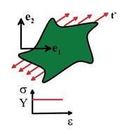
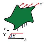
Consider a rigid perfectly plastic solid, which has mass density ${\rho }_0$, and a Von-Mises yield surface with yield stress in uniaxial tension Y. By definition, the elastic strains are zero in a rigid plastic material: the figure shows the stress-strain curve. The solid is subjected to tractions $t^{*}$ on the its boundary.  The solid may also be subjected to a body force b (per unit mass) acting on the interior of the solid.  Assume that the loading is sufficient to cause the solid to collapse.

 

 

Velocity discontinuities: Note that the velocity and stress fields in a collapsing rigid plastic solid need not necessarily be continuous.  The solution often has shear discontinuities, as illustrated below. In the picture, the top part of the solid slides relative to the bottom part.  We need a way to describe this kind of deformation.  To do so,

 

1. We assume that the velocity field $\dot{u}$ at collapse may have a finite set of such shear discontinuities, which occur over a collection of surfaces $S$.  Let m be a unit vector normal to the surface at some point , and let ${\dot{u}}^{\pm }$  ${\sigma }_{ij}^{\pm }$ denote the limiting values of velocity and stress ${\sigma }_{ij}$ on the two sides of the surface.

 

2. To ensure that no holes open up in the material, the velocity discontinuity must satisfy

$({\dot{u}}^{+}-{\dot{u}}^{-})\cdot m=0$

 

3. The solids immediately adjacent to the discontinuity exert equal and opposite forces on each other.  Therefore

${\sigma }_{ij}^{+}{m}_i={\sigma }_{ij}^{-}{m}_i$

 

4. We will use the symbol $[[\dot{u}]]$ to denote the relative velocity of sliding across the discontinuity, i.e.

$[[\dot{u}]]=\left|{\dot{u}}^{+}-{\dot{u}}^{-}\right|=\sqrt{\left({\dot{u}}_i^{+}-{\dot{u}}_i^{-}\right)\left({\dot{u}}_i^{+}-{\dot{u}}_i^{-}\right)}$

 

5. The yield criterion and plastic flow rule require that ${\sigma }_{ij}{m}_j({\dot{u}}_i^{+}-{\dot{u}}_i^{-})=Y[[u]]/\sqrt{3}$ on any surfaces of velocity discontinuity. 

 

 

Kinematically admissible collapse mechanism: The kinematically admissible collapse mechanism is analogous to the kinematically admissible displacement field that was introduced to define the potential energy of an elastic solid.  By definition, a kinematically admissible collapse mechanism is any velocity field v satisfying $\partial v_i/\partial x_i=0$ (i.e. v is volume preserving)

 

Like u, the virtual velocity v may have a finite set of discontinuities across surfaces $\widehat{S}$ with normal $\widehat{m}$ (these are not necessarily the discontinuity surfaces for the actual collapse mechanism).  We use

$[[v]]=\left|v^{+}-v^{-}\right|=\sqrt{\left(v_i^{+}-v_i^{-}\right)\left(v_i^{+}-v_i^{-}\right)}$

to denote the magnitude of the velocity discontinuity. We also define the virtual strain rate

${\widehat{\dot{\epsilon }}}_{ij}={\displaystyle \frac{1}{2}({\displaystyle \frac{\partial v_i}{\partial x_j}+{\displaystyle \frac{\partial v_j}{\partial x_i})}}}$

 (note that ${\widehat{\dot{\epsilon }}}_{kk}=0$ ) and the effective virtual plastic strain rate

${\widehat{\dot{\overline{\epsilon }}}}^p=\sqrt{2{\widehat{\dot{\epsilon }}}_{ij}{\widehat{\dot{\epsilon }}}_{ij}/3}$

 

 

Plastic Dissipation: Finally, we define the plastic dissipation associated with the virtual velocity field v as

$\Phi (v)={\displaystyle \underset{R}{\int }Y{\widehat{\dot{\overline{\epsilon }}}}^p}dV+{\displaystyle \underset{\widehat{S}}{\int }{\displaystyle \frac{Y}{\sqrt{3}}[[v]]dA}}-{\displaystyle \underset{R}{\int }{\rho }_0{b}_i{v}_{i}dA}-{\displaystyle \underset{\partial R}{\int }{t}_i^{*}{v}_{i}dA}$

 

The terms in this expression have the following physical interpretation:

 

1. The first integral represents the work dissipated in plastically straining the solid;

 

2. The second integral represents the work dissipated by plastic shearing on the velocity discontinuities;

 

3. The third integral is the rate of mechanical work done by body forces

 

4. The fourth integral is the rate of mechanical work done by the prescribed surface tractions.

 

 

 

6.3.2. The Principle of Minimum Plastic Dissipation

 

Let $\dot{u}$ denote the actual velocity field that causes a rigid plastic solid to collapse under a prescribed loading.  Let v be any kinematically admissible collapse mechanism.  Let $\Phi (v)$ denote the plastic dissipation, as defined in the preceding section.  Then

 

1. $\Phi (v)\ge \Phi (\dot{u})$

 

2. $\Phi (\dot{u})=0$

 

Thus, $\Phi$ is an absolute minimum for $v=u$ - in other words, the actual velocity field at collapse minimizes $\Phi$.  Moreover, $\Phi$ is zero for the actual collapse mechanism.

 

 

Derivation: Begin by summarizing the equations governing the actual collapse solution. Let $[{\dot{u}}_i,{\dot{\epsilon }}_{ij},{\sigma }_{ij}]$ denote the actual velocity, strain rate and stress in the solid at collapse. Let $S_{ij}={\sigma }_{ij}-{\sigma }_{kk}{\delta }_{ij}/3$ denote the deviatoric stress. The fields must satisfy governing equations and boundary conditions

 

· Strain-displacement relation ${\epsilon }_{ij}=(\partial u_i/\partial x_j+\partial u_j/\partial x_i)/2$

 

· Stress equilibrium $\partial {\sigma }_{ij}/\partial x{}_i+{\rho }_0{b}_j=0$

 

· Plastic flow rule and yield criterion

${\dot{\epsilon }}_{ij}=\left\{\begin{array}{c}{\dot{\overline{\epsilon }}}^p{\displaystyle \frac{3}{2}{\displaystyle \frac{S_{ij}}{Y}\sqrt{{\displaystyle \frac{3}{2}{S}_{ij}{S}_{ij}}}=Y}}\\ 0\sqrt{{\displaystyle \frac{3}{2}{S}_{ij}{S}_{ij}}}<Y\end{array}\right.$

On velocity discontinuities, these conditions require that ${\sigma }_{ij}{m}_j({\dot{u}}_i^{+}-{\dot{u}}_i^{-})=Y[[\dot{u}]]/\sqrt{3}$

 

· Boundary conditions

${\sigma }_{ij}{n}_i=t_j^{*}{x}_i\in \partial R$

 

 

We start by showing that $\Phi (\dot{u})=0$. 

 

1. By definition

$\Phi (\dot{u})={\displaystyle \underset{R}{\int }Y{\dot{\overline{\epsilon }}}^p}dV+{\displaystyle \underset{S}{\int }{\displaystyle \frac{Y}{\sqrt{3}}[[\dot{u}]]dA}}-{\displaystyle \underset{R}{\int }{\rho }_0{b}_i{\dot{u}}_{i}dA}-{\displaystyle \underset{\partial R}{\int }{t}_i^{*}{\dot{u}}_{i}dA}$

 

2. Note that, using (i) the flow rule, (ii) the condition that $S_{ii}=0$ and (iii) the yield criterion

${\sigma }_{ij}{\dot{\epsilon }}_{ij}^p={\sigma }_{ij}{\dot{\overline{\epsilon }}}^p{\displaystyle \frac{3}{2}{\displaystyle \frac{S_{ij}}{Y}=(S_{ij}+{\sigma }_{kk}{\delta }_{ij}){\dot{\overline{\epsilon }}}^p{\displaystyle \frac{3}{2}{\displaystyle \frac{S_{ij}}{Y}={\dot{\overline{\epsilon }}}^p{\displaystyle \frac{3}{2}{\displaystyle \frac{S_{ij}{S}_{ij}}{Y}=Y{\dot{\overline{\epsilon }}}^p}}}}}}$

 

3. Note that ${\sigma }_{ij}{\dot{\epsilon }}_{ij}={\sigma }_{ij}(\partial u_i/\partial x_j+\partial u_j/\partial x_i)/2={\sigma }_{ij}\partial u_j/\partial x_i$ from the symmetry of ${\sigma }_{ij}$. Hence

${\displaystyle \underset{R}{\int }Y{\dot{\overline{\epsilon }}}^p}dV={\displaystyle \underset{R}{\int }{\sigma }_{ij}{\dot{\epsilon }}_{ij}dV}={\displaystyle \underset{R}{\int }{\sigma }_{ij}\partial {\dot{u}}_j/\partial x_{i}dV}$

 

4. Note that ${\sigma }_{ij}\partial u_j/\partial x_i=\partial ({\sigma }_{ij}{u}_j)/\partial x_i-\left(\partial {\sigma }_{ij}/\partial x_i\right){\dot{u}}_j$.  Substitute into the expression for $\Phi (u)$, combine the two volume integrals and recall (equilibrium) that $\partial {\sigma }_{ij}/\partial x_i+{\rho }_0{b}_j=0$ to see that

$\Phi (\dot{u})={\displaystyle \underset{R}{\int }\partial \left({\sigma }_{ij}{\dot{u}}_j\right)/\partial x_i}dV+{\displaystyle \underset{S}{\int }{\displaystyle \frac{Y}{\sqrt{3}}[[\dot{u}]]dA}}-{\displaystyle \underset{\partial R}{\int }{t}_i^{*}{\dot{u}}_{i}dA}$

 

5. Apply the divergence theorem to the volume integral in this result.  When doing so, note that we must include contributions from the velocity discontinuity across S as follows

$\Phi (\dot{u})={\displaystyle \underset{\partial R}{\int }{\sigma }_{ij}{\dot{u}}_j{n}_i}dA+{\displaystyle \underset{S}{\int }{\sigma }_{ij}{\dot{u}}_j^{+}{n}_i^{+}}dA+{\displaystyle \underset{S}{\int }{\sigma }_{ij}{\dot{u}}_j^{-}{n}_i^{-}}dA+{\displaystyle \underset{S}{\int }{\displaystyle \frac{Y}{\sqrt{3}}[[\dot{u}]]dA}}-{\displaystyle \underset{\partial R}{\int }{t}_i^{*}{\dot{u}}_{i}dA}$

 

6. Finally, recall that ${\sigma }_{ij}{n}_i=t_j^{*}$ on the boundary, and note that the outward normals to the solids adjacent to S are related to m  by $n_i^{+}=-m_i$ $n_i^{-}=m_i$ (see the figure). Thus

$\Phi (\dot{u})=-{\displaystyle \underset{S}{\int }{\sigma }_{ij}({\dot{u}}_j^{+}-{\dot{u}}_j^{-})m_i}dA+{\displaystyle \underset{S}{\int }{\displaystyle \frac{Y}{\sqrt{3}}[[\dot{u}]]dA}}$

Since ${\sigma }_{ij}{m}_j({\dot{u}}_i^{+}-{\dot{u}}_i^{-})=Y[[u]]/\sqrt{3}$, we find that $\Phi (u)=0$ as required.

 

 

Next, we show that $\Phi (v)\ge 0$.  To this end,

 

1. Let $v_i$ be a kinematically admissible velocity field as defined in the preceding section, with strain rate

${\widehat{\dot{\epsilon }}}_{ij}={\displaystyle \frac{1}{2}({\displaystyle \frac{\partial v_i}{\partial x_j}+{\displaystyle \frac{\partial v_j}{\partial x_i})}}}$

 

2. Let ${\widehat{S}}_{ij}$ be the stress necessary to drive the kinematically admissible collapse mechanism, which must satisfy the plastic flow rule and the yield criterion

${\widehat{\dot{\epsilon }}}_{ij}=\widehat{\dot{\overline{\epsilon }}}{\displaystyle \frac{3}{2}{\displaystyle \frac{{\widehat{S}}_{ij}}{Y}\sqrt{3{\widehat{S}}_{ij}{\widehat{S}}_{ij}/2}=Y}}$

 

3. Recall that the plastic strains and stresses associated with the kinematically admissible field must satisfy the Principle of Maximum Plastic Resistance (Section 3.7.10), which in the present context implies that

$\left({\widehat{\sigma }}_{ij}-{\sigma }_{ij}\right){\widehat{\dot{\epsilon }}}_{ij}\ge 0$

To see this, note that ${\widehat{\sigma }}_{ij}$ is the stress required to cause the plastic strain rate  ${\widehat{\dot{\epsilon }}}_{ij}$, while the actual stress state at collapse ${\sigma }_{ij}$ must satisfy $\sqrt{3S_{ij}{S}_{ij}/2}\le Y$.

 

4. Note that ${\widehat{\sigma }}_{ij}{\widehat{\dot{\epsilon }}}_{ij}=\left({\widehat{S}}_{ij}+{\widehat{\sigma }}_{kk}{\delta }_{ij}\right)d{\widehat{\dot{\overline{\epsilon }}}}^{p}3{\widehat{S}}_{ij}/2Y=Yd{\widehat{\dot{\overline{\epsilon }}}}^p$.  Substituting into the principle of maximum plastic resistance and integrating over the volume of the solid shows that

${\displaystyle \underset{R}{\int }Y{\widehat{\dot{\overline{\epsilon }}}}^{p}dV}-{\displaystyle \underset{R}{\int }{\sigma }_{ij}{\widehat{\dot{\epsilon }}}_{ij}dV}\ge 0$

 

5. Next, note that

${\sigma }_{ij}{\widehat{\dot{\epsilon }}}_{ij}={\sigma }_{ij}\left(\partial v_i/\partial x_j+\partial v_j/\partial x_i\right)/2={\sigma }_{ij}\partial v_j/\partial x_i=\partial \left({\sigma }_{ij}{v}_j\right)/\partial x_i-\left(\partial {\sigma }_{ij}/\partial x_i\right)v_j$

 

6. The equilibrium equation shows that $\partial {\sigma }_{ij}/\partial x_i=-{\rho }_0{b}_j$.  Substituting this into the result of (5) and then substituting into the result of (4) shows that

${\displaystyle \underset{R}{\int }Y{\widehat{\dot{\overline{\epsilon }}}}^{p}dV}-{\displaystyle \underset{R}{\int }\partial \left({\sigma }_{ij}{v}_j\right)/\partial x_{i}dV}-{\displaystyle \underset{R}{\int }{\rho }_0{b}_j{v}_{j}dV}\ge 0$

 

7. Apply the divergence theorem to the second integral. When doing so, note that we must include contributions from the velocity discontinuity across $\widehat{S}$ as follows

${\displaystyle \underset{R}{\int }Y{\widehat{\dot{\overline{\epsilon }}}}^{p}dV}-{\displaystyle \underset{\widehat{S}}{\int }{\sigma }_{ij}{v}_j{n}_i^{+}dA}-{\displaystyle \underset{\widehat{S}}{\int }{\sigma }_{ij}{v}_j{n}_i^{-}dA}-{\displaystyle \underset{\partial R}{\int }{\sigma }_{ij}{v}_j{n}_{i}dA}-{\displaystyle \underset{R}{\int }{\rho }_0{b}_j{v}_{j}dV}\ge 0$

 

8. Recall that ${\sigma }_{ij}{n}_i=t_j^{*}$ on the boundary, and note that the outward normals to the solids adjacent to S are related to m  by $n_i^{+}=-m_i$ $n_i^{-}=m_i$.  Thus

${\displaystyle \underset{R}{\int }Y{\widehat{\dot{\overline{\epsilon }}}}^{p}dV}+{\displaystyle \underset{\widehat{S}}{\int }{\sigma }_{ij}{\widehat{m}}_j(v_i^{+}-v_i^{-})dA-{\displaystyle \underset{R}{\int }{b}_i{v}_{i}dV}-{\displaystyle \underset{{\partial }_{2}R}{\int }{t}_i^{*}{v}_{i}dA}}\ge 0$

 

9. Finally, note that on $\widehat{S}$

${\sigma }_{ij}{\widehat{m}}_j(v_i^{+}-v_i^{-})\le Y[[v]]/\sqrt{3}$

since the shear stress acting on any plane in the solid cannot exceed $Y/\sqrt{3}$.  Thus

${\displaystyle \underset{R}{\int }Y{\widehat{\dot{\overline{\epsilon }}}}^{p}dV}+{\displaystyle \underset{\widehat{S}}{\int }Y[[v]]/\sqrt{3}dA-{\displaystyle \underset{R}{\int }{b}_i{v}_{i}dV}-{\displaystyle \underset{{\partial }_{2}R}{\int }{t}_i^{*}{v}_{i}dA}}\ge 0$

 proving that $\Phi (v)\ge 0$ as required.

 

 

 

6.3.3 The Upper Bound Plastic Collapse Theorem

 

Consider a rigid plastic solid, subjected to some distribution of tractions $t_i^{*}$ and body forces $b_i$ as shown in the figure. We will attempt to estimate the factor $\beta$ by which the loading can be increased before the solid collapses ( $\beta$ is effectively the factor of safety).  We suppose that the solid will collapse for loading $\beta t_i^{*}$, $\beta b_i$.

 

To estimate $\beta$, we guess the mechanism of collapse.  The collapse mechanism will be an admissible velocity field, which may have a finite set of discontinuities across surfaces $\widehat{S}$ with normal $\widehat{m}$, as discussed in Section 6.2.1.

 

The principle of minimum plastic dissipation then states that

${\displaystyle \underset{R}{\int }Y{\widehat{\dot{\overline{\epsilon }}}}^{p}dV}+{\displaystyle \underset{\widehat{S}}{\int }{\sigma }_{ij}{\widehat{m}}_j(v_i^{+}-v_i^{-})dA-{\displaystyle \underset{R}{\int }\beta b_i{v}_{i}dV}-{\displaystyle \underset{\partial R}{\int }\beta t_i^{*}{v}_{i}dA}}\ge 0$

for any collapse mechanism, with equality for the true mechanism of collapse. Therefore

$\beta \le {\displaystyle \frac{{\displaystyle \underset{R}{\int }Y{\widehat{\dot{\overline{\epsilon }}}}^p}dV+{\displaystyle \underset{\widehat{S}}{\int }Y[[v]]/\sqrt{3}dA}}{{\displaystyle \underset{R}{\int }{b}_i{v}_{i}dA}+{\displaystyle \underset{\partial R}{\int }{t}_i^{*}{v}_{i}dA}}}$

 

Expressed in words, this equation states that we can obtain an upper bound to the collapse loads by postulating a collapse mechanism, and computing the ratio of the plastic dissipation associated with this mechanism to the work done by the applied loads. 

 

So, we can choose any collapse mechanism, and use it to estimate a safety factor.  The actual safety factor is likely to be lower than our estimate (it will be equal if we guessed right).  This method is evidently inherently unsafe, since it overestimates the safety factor $–$ but it is usually possible guess the collapse mechanism quite accurately, and so with practice you can get excellent estimates.

 

 

 

6.3.4 Examples of applications of the upper bound theorem

 

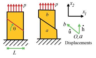
Example 1: collapse load for a uniaxial bar. We will illustrate the bounding theorems using a few examples.  First, we will compute  bounds to the collapse load for a uniaxial bar.  Assume the bar has unit out of plane thickness, for simplicity.

 

To get an upper bound, we guess a collapse mechanism as shown below. The top and bottom half of the bar slide past each other as rigid blocks, as shown, with a velocity discontinuity across the line shown in red.

 

 

The upper bound theorem gives

$\beta \le {\displaystyle \frac{{\displaystyle \underset{R}{\int }Y{\widehat{\dot{\overline{\epsilon }}}}^p}dV+{\displaystyle \underset{\widehat{S}}{\int }Y[[v]]/\sqrt{3}dA}}{{\displaystyle \underset{R}{\int }{b}_i{v}_{i}dA}+{\displaystyle \underset{\partial R}{\int }{t}_i^{*}{v}_{i}dA}}}$

In this problem the strain rate vanishes, since we assume the two halves of the bar are rigid.  The plastic dissipation is

${\displaystyle \underset{\widehat{S}}{\int }Y[[v]]/\sqrt{3}dA}=Y(\dot{h}/\sin \theta )(L/\cos \theta )/\sqrt{3}$

The body force vanishes, and

${\displaystyle \underset{\partial R}{\int }{t}_i^{*}{\dot{u}}_i}dA=pL\dot{h}$

where $\dot{h}$ is the vertical component of the velocity of the top block.  Thus

$\beta p\le 2Y/(\sqrt{3}\sin 2\theta )$

The best upper bound occurs for $\theta =\pi /4$, giving $\beta p\le 2Y/\sqrt{3}$ for the collapse load.

 

 

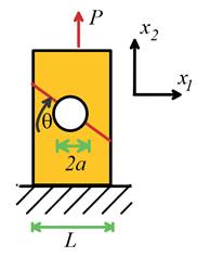
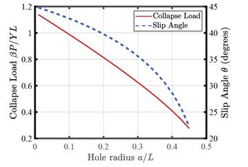
Example 2: Collapse load for a bar containing a hole. For a slightly more interesting problem, consider the effect of inserting a hole with radius a in the center of the column, as shown below. This time we apply a force to the top of the column, rather than specify the traction distribution in detail.  We will accept any solution that has traction acting on the top surface that is statically equivalent to the applied force.

 

 

A possible collapse mechanism is shown above.  The plastic dissipation is

${\displaystyle \underset{\widehat{S}}{\int }Y[[v]]/\sqrt{3}dA}=\left(Y/\sqrt{3}\right)(\dot{h}/\sin \theta )(L/\cos \theta -2a)$

The rate of work done by the applied loading is

${\displaystyle \underset{\partial R}{\int }{t}_i^{*}{\dot{u}}_i}dA=P\dot{h}$

Our upper bound follows as

$\beta P\le Y(L/\cos \theta -2a)/(\sqrt{3}\sin \theta )$

The best upper bound follows by minimizing this result with respect to $\theta$.  The minimizing angle and the corresponding upper bound to the collapse load are plotted below.   Of course, this is an upper bound.  You should be able to find collapse mechanisms that give lower collapse loads!

 

 

Example 3: Force required to indent a rigid platic surface. For our next example, we attempt to find upper and lower bounds to the force required to push a flat plane punch into a rigid plastic solid.  This problem is interesting because an exact solution exists, so we can assess the accuracy of the bounding calculations.

 

 

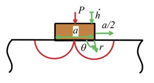
A possible collapse mechanism is shown above. In each semicircular region we assume a constant circumferential velocity $v_{\theta }=\dot{h}$.  To compute the plastic dissipation in one of the regions, adopt a cylindrical-polar coordinate system with origin at the edge of the contact.  The strain distribution follows as

$\begin{array}{l}{\dot{\epsilon }}_{rr}={\dot{\epsilon }}_{\theta \theta }=0{\dot{\epsilon }}_{r\theta }={\displaystyle \frac{1}{2}{\displaystyle \frac{v_{\theta }}{r}={\displaystyle \frac{\dot{h}}{2r}}}}\\ \Rightarrow {\widehat{\dot{\overline{\epsilon }}}}^p=\sqrt{{\displaystyle \frac{2}{3}{\widehat{\dot{\epsilon }}}_{ij}{\widehat{\dot{\epsilon }}}_{ij}}}={\displaystyle \frac{\dot{h}}{r\sqrt{3}}}\end{array}$

Thus the plastic dissipation is

${\displaystyle \underset{R}{\int }Y{\widehat{\dot{\overline{\epsilon }}}}^p}dV+{\displaystyle \underset{\widehat{S}}{\int }Y[[v]]/\sqrt{3}dA}=2\left\{{\displaystyle \underset{0}{\overset{\pi }{\int }}{\displaystyle \underset{0}{\overset{a/2}{\int }}Y{\displaystyle \frac{\dot{h}}{r\sqrt{3}}}}}rdrd\theta +{\displaystyle \frac{Y}{2\sqrt{3}}\dot{h}\pi a}\right\}={\displaystyle \frac{2\pi }{\sqrt{3}}\dot{h}Ya}$

(note that there’s a velocity discontinuity at r=a). The work done by applied loading is just $\dot{h}P$ giving the upper bound

$\beta P\le 2\pi Ya/\sqrt{3}$

The exact solution to this problem was given in Section 6.2.1 as

$\beta P=(\pi +2)Ya/\sqrt{3}$

The error is 17% - close enough for government work.

 

 

 

 Example 4: The figure below shows a simple model of machining.  The objective is to determine the horizontal force P acting on the tool (or workpiece) in terms of the depth of cut h, the tool rake angle $\alpha$ and the shear yield stress of the material $Y$

 

 

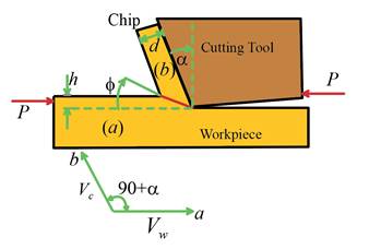
To perform the calculation, we adopt a reference frame that moves with the tool.  Thus, the tool appears stationary, while the workpiece moves at speed $V_w$ to the right.  The collapse mechanism consists of shear across the red line shown in the picture.

 

Elementary geometry gives the chip thickness d as

$d=h{\displaystyle \frac{\cos \left(\varphi +\alpha \right)}{\sin \varphi }}$

Mass conservation (material flowing into slip discontinuity = material flowing out of slip discontinuity) gives the velocity of material in the chip $V_c$ as

$V_c=V_w{\displaystyle \frac{h}{d}=V_w{\displaystyle \frac{\sin \varphi }{\cos \left(\varphi +\alpha \right)}}}$

The velocity discontinuity across the shear band is

$\begin{array}{l}\left|V_{ba}\right|=\sqrt{V_w^2+V_c^2+2V_c{V}_w\sin \alpha }\\ =V_w\sqrt{1+{\displaystyle \frac{{\sin }^2\varphi }{{\cos }^2\left(\varphi +\alpha \right)}+2\sin \alpha {\displaystyle \frac{\sin \varphi }{\cos \left(\varphi +\alpha \right)}}}}\end{array}$

The plastic dissipation follows as

${\dot{W}}^P={\displaystyle \frac{h}{\sin \varphi }\left|V_{ab}\right|{\displaystyle \frac{Y}{\sqrt{3}}}}$

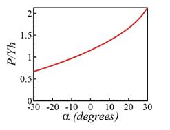
The upper bound theorem gives

$\begin{array}{l}P{V}_w\le {\displaystyle \frac{h}{\sin \varphi }\left|V_{ab}\right|{\displaystyle \frac{Y}{\sqrt{3}}}}\\ \Rightarrow P\le {\displaystyle \frac{hY}{\sqrt{3}\sin \varphi }\sqrt{1+{\displaystyle \frac{{\sin }^2\varphi }{{\cos }^2\left(\varphi +\alpha \right)}+2\sin \alpha {\displaystyle \frac{\sin \varphi }{\cos \left(\varphi +\alpha \right)}}}}}\end{array}$

To obtain the best estimate for P, we need to minimize the right hand side of this expression with respect to $\varphi$.  This gives

$\varphi ={\tan }^{-1}(1-\tan (\alpha ))$

The resulting upper bound to the machining force is plotted below

 

 

 

6.3.5 The Lower Bound Plastic Collapse Theorem

 

The lower bound theorem provides a safe estimate of the collapse loads for a rigid plastic solid.

 

Consider a rigid plastic solid, subjected to some distribution of tractions $t_i^{*}$ and body forces $b_i$, as shown in the figure. We will attempt to estimate the factor $\beta$ by which the loading can be increased before the solid collapses ( $\beta$ is effectively the factor of safety).  We suppose that the solid will collapse for loading $\beta t_i^{*}$, $\beta b_i$.

 

To estimate $\beta$, we guess the distribution of stress in the solid at collapse.

 

We will denote the guess for the stress distribution by ${\widehat{\sigma }}_{ij}$.  The stress distribution must

 

1. Satisfy the boundary conditions ${\widehat{\sigma }}_{ij}{n}_j={\beta }_L{t}_i^{*}$, where ${\beta }_L$ is a lower bound to $\beta$

 

2. Satisfy the equations of equilibrium $\partial {\widehat{\sigma }}_{ij}/\partial x_j+{\beta }_L{b}_i=0$ within the solid,

 

3. Must not violate the yield criterion anywhere within the solid, $f({\widehat{\sigma }}_{ij})\le 0$

 

The lower bound theorem states that if any such stress distribution can be found, the solid will not collapse, i.e. ${\beta }_L\le \beta$.

 

 

Derivation

 

1. Let $[{\dot{u}}_i,{\dot{\epsilon }}_{ij},{\sigma }_{ij}]$ denote the actual velocity field in the solid at collapse.  These must satisfy the field equations and constitutive equations listed in Section 6.3.1.

 

2. Let ${\widehat{\sigma }}_{ij}$ denote the guess for the stress field.

 

3. The Principle of Maximum Plastic Resistance (see Section 3.7.10) shows that $\left({\sigma }_{ij}-{\widehat{\sigma }}_{ij}\right){\dot{\epsilon }}_{ij}\ge 0$, since ${\widehat{\sigma }}_{ij}$ is at or below yield.

 

4. Integrating this equation over the volume of the solid, and using the principle of virtual work on the two terms shows that

$\begin{array}{l}{\displaystyle \underset{V}{\int }\left({\sigma }_{ij}-{\widehat{\sigma }}_{ij}\right){\dot{\epsilon }}_{ij}dV={\displaystyle \underset{\partial V}{\int }{\sigma }_{ij}{n}_j{\dot{u}}_{i}dA}-{\displaystyle \underset{\partial V}{\int }{\widehat{\sigma }}_{ij}{n}_j{\dot{u}}_i}dA}\ge 0\\ \Rightarrow \beta {\displaystyle \underset{\partial V}{\int }{t}_i{\dot{u}}_i}dA\ge {\beta }_L{\displaystyle \underset{\partial V}{\int }{t}_i{\dot{u}}_{i}dA}\end{array}$

 This proves the theorem.

 

 

 

6.3.6 Examples of applications of the lower bound plastic collapse theorem

 

 

Example 1: Collapse load for a plate containing a hole.  A plate with width L contains a hole of radius a at its center, as shown in the figure. The plate is subjected to a tensile force P as shown (the traction distribution is not specified in detail we will accept any solution that has traction acting on the top surface that is statically equivalent to the applied force).

 

 

For a statically admissible stress distribution, we consider the stress field shown in Fig. 6.40, with ${\sigma }_{22}=0\left|x_1\right|<a{\sigma }_{22}=Y\left|x_1\right|>a$, and all other stress components zero.

 

The estimate for the applied load at collapse follows as ${\beta }_{L}P=2Y(L-a)$

 

 

 

Example 2: Rigid indenter in contact with a half-space.  We consider a flat indenter with width a that is pushed into the surface of a half-space by a force P.  The stress state illustrated below will be used to obtain a lower bound to the collapse load in the solid.  

 

 

 

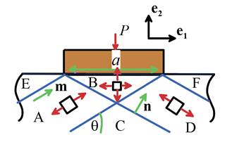
Note that

 

1. Regions C, E, F are stress free

 

2. The stress in regions A and D consists of a state of uniaxial stress, with direction parallel to the boundaries between AC (or AE) and CD (or DF) respectively.  We will denote this stress by ${\sigma }^{A}m\otimes m$, where m is a unit vector parallel to the direction of the uniaxial stress.

 

3. The stress state in the triangular region B has principal directions of stress parallel to $e_{\alpha }$. We will write this stress state as ${\sigma }_{11}^B{e}_1\otimes e_1+{\sigma }_{22}^B{e}_2\otimes e_2$

 

 

The stresses in each region must be chosen to satisfy equilibrium, and to ensure that the stress is below yield everywhere.   The stress is constant in each region, so equilibrium is satisfied locally.  However, the stresses are discontinuous across AC, AB, etc.  To satisfy equilibrium, equal and opposite tractions must act on the material surfaces adjacent to the discontinuity, which requires, e.g. that ${\sigma }_{ij}^A{n}_j={\sigma }_{ij}^B{n}_j$, where n is a unit vector normal to the boundary between A and B as indicated in Figure 6.41.  We enforce this condition as follows:

 

1. Note that $m=\cos \theta e_1+\sin \theta e_2$ $n=\sin \theta e_1+\cos \theta e_2$

 

2. Equilibrium across the boundary between A and B requires

$\begin{array}{l}{\sigma }^A\left(m\otimes m\right)\cdot n=\left({\sigma }_{11}^B{e}_1\otimes e_1+{\sigma }_{22}^B{e}_2\otimes e_2\right)\cdot n\\ \Rightarrow {\sigma }^A\left(\cos \theta e_1+\sin \theta e_2\right)2\sin \theta \cos \theta ={\sigma }_{11}^B{e}_1\sin \theta +{\sigma }_{22}^B{e}_2\cos \theta \\ \Rightarrow {\sigma }_{11}^B=2{\sigma }^A{\cos }^2\theta {\sigma }_{22}^B=2{\sigma }^A{\sin }^2\theta \end{array}$

 

3. We must now choose ${\sigma }^A$ and $\theta$ to maximize the collapse load, while ensuring that the stresses do not exceed yield in regions A or B.   Clearly, this requires ${\sigma }^A=-Y$; while $\theta$ must be chosen to ensure that $\left|{\sigma }_{22}^B-{\sigma }_{11}^B\right|<Y$.  This requires $1/2<\cos \theta <\sqrt{3}/2$.   The largest value for $\theta$ maximizes the bound.

 

4. Finally, substituting for $\theta$ gives ${\sigma }_{22}^B=-3Y/2$.  We see that the lower bound is $P=-3Ya/2$.

  

 

 

6.3.7 The lower bound shakedown theorem

 

In this and the next section we derive two important theorems that can be used to estimate the maximum cyclic loads that can be imposed on a component without exceeding yield.  The concept of shakedown in a solid subjected to cyclic loads was introduced in Section 6.1.4, which discussed the behavior of a spherical shell subjected to cyclic internal pressure.   It was shown that, if the first cycle of pressure exceeds yield, residual stresses are introduced into the shell, which may prevent further plastic deformation under subsequent load cycles.  This process is known as shakedown, and the maximum load for which it can occur is known as the shakedown limit. 

 

We proceed to derive a theorem that can be used to obtain a safe estimate to the maximum cyclic load that can be applied to a structure without inducing cyclic plastic deformation.

 

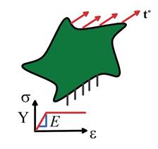We consider an elastic-perfectly plastic solid, sketched in the figure. The solid has Young’s modulus E, Poisson’s ratio $\nu$ and has a Von-Mises yield surface with uniaxial tensile yield stress Y, and an associated flow law. Assume that

 

1. The displacement $u=0$ on part of the boundary of the solid ${\partial }_{1}R$

 

2. The remainder of the boundary  ${\partial }_{2}R$ is subjected to a prescribed cycle of traction $t^{*}(t)$.   The history of traction is periodic, with a period T.

 

 

Define the following quantities:

 

1. Let $[u_i,{\epsilon }_{ij},{\sigma }_{ij}]$ denote the actual history of displacement, strain and stress induced in the solid by the applied loading.  The strain is partitioned into elastic and plastic parts as ${\epsilon }_{ij}={\epsilon }_{ij}^e+{\epsilon }_{ij}^p$

 

2. Let $[u_i^{\epsilon },{\epsilon }_{ij}^{\epsilon },{\sigma }_{ij}^{\epsilon }]$ denote the history of displacement, strain and stress induced by the prescribed traction in a perfectly elastic solid with identical geometry.

 

3. We introduce (time dependent) residual stress ${\rho }_{ij}$ and residual strain ${\gamma }_{ij}$ fields, which (by definition) satisfy

${\sigma }_{ij}={\sigma }_{ij}^{\epsilon }+{\rho }_{ij}{\epsilon }_{ij}={\epsilon }_{ij}^e+{\epsilon }_{ij}^p={\epsilon }_{ij}^{\epsilon }+{\gamma }_{ij}+{\epsilon }_{ij}^p$

Note that, (i) because ${\sigma }_{ij}^{\epsilon }{n}_j={\sigma }_{ij}{n}_j=t_i^{*}$ on ${\partial }_{2}R$, it follows that ${\rho }_{ij}{n}_j=0$ on  ${\partial }_{2}R$; and (ii) because $\partial {\sigma }_{ij}^{\epsilon }/\partial x_j=\partial {\sigma }_{ij}/\partial x_j=0$ it follows that $\partial {\rho }_{ij}/\partial x_j=0$

 

 

The lower bound shakedown theorem can be stated as follows: The solid is guaranteed to shake down if any time independent residual stress field ${\overline{\rho }}_{ij}$ can be found which satisfies:

 

· The equilibrium equation $\partial {\overline{\rho }}_{ij}/\partial x_j=0$;

 

· The boundary condition ${\overline{\rho }}_{ij}{n}_j=0$ on  ${\partial }_{2}R$;

 

· When the residual stress is combined with the elastic solution, the combined stress does not exceed yield $f({\sigma }_{ij}^{\epsilon }+{\overline{\rho }}_{ij})\le 0$ at any time during the cycle of load.

 

 

The theorem is valuable because shakedown limits can be estimated using the elastic solution, which is much easier to calculate than the elastic-plastic solution. 

 

Proof of the lower bound theorem:  The proof is one of the most devious in all of solid mechanics. 

 

1. Consider the strain energy associated with the difference between the actual residual stress field ${\rho }_{ij}$, and the guess for the residual stress field ${\overline{\rho }}_{ij}$, which can be calculated as

$W={\displaystyle \frac{1}{2}{\displaystyle \underset{R}{\int }{S}_{ijkl}({\rho }_{ij}-{\overline{\rho }}_{ij})({\rho }_{kl}-{\overline{\rho }}_{kl})}dV}$

where $S_{ijkl}$ is the elastic compliance tensor.   For later reference note that W has to be positive, because strain energy density is always positive or zero.

 

2. The rate of change of W can be calculated as

${\displaystyle \frac{dW}{dt}={\displaystyle \underset{R}{\int }{S}_{ijkl}({\rho }_{ij}-{\overline{\rho }}_{ij}){\displaystyle \frac{d{\rho }_{kl}}{dt}}}dV\ge 0}$

(to see this, recall that $S_{ijkl}=S_{klij}$ )

 

3. Note that $S_{ijkl}{\rho }_{kl}={\gamma }_{ij}={\epsilon }_{ij}-{\epsilon }_{ij}^p-{\epsilon }_{ij}^{\epsilon }$. Consequently, we see that

${\displaystyle \frac{dW}{dt}=-{\displaystyle \underset{R}{\int }({\rho }_{ij}-{\overline{\rho }}_{ij}){\displaystyle \frac{d{\epsilon }_{ij}^p}{dt}}}dV+{\displaystyle \underset{R}{\int }({\rho }_{ij}-{\overline{\rho }}_{ij})\left({\displaystyle \frac{d{\epsilon }_{ij}}{dt}-{\displaystyle \frac{d{\epsilon }_{ij}^{\epsilon }}{dt}}}\right)}dV\ge 0}$

 

4. Using the principle of virtual work, the second integral can be expressed as an integral over the boundary of the solid

${\displaystyle \underset{A}{\int }({\rho }_{ij}-{\overline{\rho }}_{ij})n_j\left({\displaystyle \frac{d{u}_i}{dt}-{\displaystyle \frac{d{u}_i^{\epsilon }}{dt}}}\right)}dA=0$

To see this, note that $({\rho }_{ij}-{\overline{\rho }}_{ij})n_j=0$ on ${\partial }_{2}R$, while ${\dot{u}}_i-{\dot{u}}_i^{\epsilon }=0$ on ${\partial }_{1}R$

 

5. The remaining integral in (3) can be re-written as

${\displaystyle \frac{dW}{dt}=-{\displaystyle \underset{R}{\int }({\rho }_{ij}-{\overline{\rho }}_{ij}){\displaystyle \frac{d{\epsilon }_{ij}^p}{dt}}}dV=-{\displaystyle \underset{R}{\int }\left[{\sigma }_{ij}-({\sigma }_{ij}^{\epsilon }+{\overline{\rho }}_{ij})\right]{\displaystyle \frac{d{\epsilon }_{ij}^p}{dt}}}dV\ge 0}$

 

6. Finally, recall that ${\sigma }_{ij}^{\epsilon }+{\overline{\rho }}_{ij}$ lies at or below yield, while ${\sigma }_{ij}$ is at yield and is the stress corresponding to the plastic strain rate ${\dot{\epsilon }}_{ij}^p$.   The principle of maximum plastic resistance therefore shows that $\left[{\sigma }_{ij}-({\sigma }_{ij}^{\epsilon }+{\overline{\rho }}_{ij})\right]{\dot{\epsilon }}_{ij}^p\ge 0$.  This inequality and  $dW/dt\ge 0$ can only be satisfied simultaneously if $\left[{\sigma }_{ij}-({\sigma }_{ij}^{\epsilon }+{\overline{\rho }}_{ij})\right]{\dot{\epsilon }}_{ij}^p=0$.  We conclude that either the plastic strain rate vanishes, or $\left[{\sigma }_{ij}-({\sigma }_{ij}^{\epsilon }+{\overline{\rho }}_{ij})\right]=0$.  In either case the solid must shake down to an elastic state.

 

 

 

6.3.8 Examples of applications of the lower bound shakedown theorem

 

 

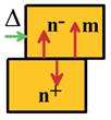
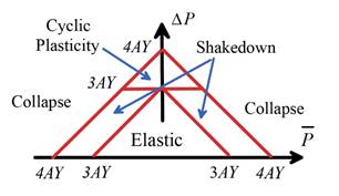
Example 1: A simple 3 bar problem.  It is traditional to illustrate the concept of shakedown using this problem.  Consider a structure made of three parallel elastic-plastic bars, with Young’s modulus E and cross sectional are A, as shown in the figure.  The two bars labeled 1 and 2 have yield stress Y; the central bar (labeled 3) has yield stress 2Y.  The structure is subjected to a cyclic load with mean value $\overline{P}$ and amplitude $\Delta P$.

 

The elastic limit for the structure is $\overline{P}\pm \Delta P=3AY$; the collapse load is $\overline{P}\pm \Delta P=4AY$.

 

To obtain a lower bound to the shakedown limit, we must

 

1. Calculate the elastic stresses in the structure $–$ the axial stress in each bar is ${\sigma }^{\epsilon }=P/3A$

 

2. Find a residual stress distribution in the structure, which satisfies equilibrium and boundary conditions, and which can be added to the elastic stresses to bring them below yield.   A suitable residual stress distribution consists of an axial stress ${\rho }^{(1)}={\rho }^{(2)}={\rho }_0,{\rho }^{(3)}=-2{\rho }_0$ in bars 1, 2 and 3. To prevent yield at the maximum and minimum load in all three bars, we require

$\begin{array}{l}-Y<(\overline{P}-\Delta P)/3A+{\rho }_0(\overline{P}+\Delta P)/3A+{\rho }_0<Y\\ -2Y<(\overline{P}-\Delta P)/3A-2{\rho }_0(\overline{P}+\Delta P)/3A-2{\rho }_0<2Y\end{array}$

The first two equations show that $\Delta P<Y$, irrespective of ${\rho }_0$.  To avoid yield in all bars at the maximum load, we must choose ${\rho }_0=-Y/3$, which gives $P+\Delta P<4AY$. Similarly, to avoid yield in all bars at the minimum load, we must choose ${\rho }_0=Y/3$, showing that $-4AY<(\overline{P}-\Delta P)$.

 

The various regimes of behavior are summarized in the figure below.

 

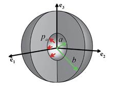Example 2: Shakedown limit for a pressurized spherical shell.  We consider an elastic-perfectly plastic thick-walled shell, with inner radius a and outer radius b.  The inner wall of the shell is subjected to a cyclic pressure, with minimum value zero, and maximum value $p_a$, as sketched in the figure

 

 

To estimate the shakedown limit we must

 

1. Calculate the stresses induced by the pressure in an elastic shell.  The solution can be found in Section 6.1.4. 

 

${\sigma }_{RR}={\displaystyle \frac{p_a{a}^3}{\left(b^3-a^3\right)}\left(1-{\displaystyle \frac{b^3}{R^3}}\right)}$  ${\sigma }_{\theta \theta }={\sigma }_{\varphi \varphi }={\displaystyle \frac{p_a{a}^3}{\left(b^3-a^3\right)}\left(1+{\displaystyle \frac{b^3}{2R^3}}\right)}$

 

2. Find a self-equilibrating residual stress field, which satisfies traction free boundary conditions on R=a, R=b, and which can be added to the elastic stresses to prevent yield in the sphere.  The equilibrium equation for the residual stress can be written

${\displaystyle \frac{d{\rho }_{RR}}{dR}+{\displaystyle \frac{1}{R}\left(2{\rho }_{RR}-{\rho }_{\theta \theta }-{\rho }_{\varphi \varphi }\right)=0}}$

We can satisfy this equation by choosing any suitable distribution for ${\rho }_{RR}$ and calculating the corresponding ${\rho }_{\theta \theta }$.  For example, we can choose ${\rho }_{RR}={\rho }_0(1-a/R)(1-b/R)$, which corresponds to ${\rho }_{\theta \theta }={\rho }_0(1-(b+a)/2R)$.  To avoid yield at maximum load, we must ensure that $\left|{\sigma }_{RR}-{\sigma }_{\theta \theta }+{\rho }_{RR}-{\rho }_{\theta \theta }\right|\le Y$, while to avoid yield at zero load, $\left|{\rho }_{RR}-{\rho }_{\theta \theta }\right|\le Y$ throughout the shell.   The critically stressed material element lies at R=a at both the maximum and zero loads, which shows that

${\displaystyle \frac{3p_a{b}^3}{(b^3-a^3)}+{\rho }_0{\displaystyle \frac{(b-a)}{2a}<Y-Y<{\rho }_0{\displaystyle \frac{(b-a)}{2a}<Y}}}$

Clearly, the best choice of ${\rho }_0$ is ${\rho }_0=-2Ya/(b-a)$

 

The estimate for the shakedown limit therefore follows as $p_a/Y<4(1-a^3/b^3)/3$.  This is equal to the exact solution derived (with considerably more effort) in Section 6.1.4.

 

 

 

6.3.9 The Upper Bound Shakedown Theorem

 

In this section we derive a theorem that can be used to obtain an over-estimate to the maximum cyclic load that can be applied to a structure without inducing cyclic plastic deformation.  Although the estimate is inherently unsafe, the theorem is easier to use than the lower bound theorem.

 

We consider an elastic-perfectly plastic solid, sketched in the figure. The solid has Young’s modulus E, Poisson’s ratio $\nu$ and has a Von-Mises yield surface with uniaxial tensile yield stress Y, and an associated flow law. Assume that

 

1. The displacement $u=0$ on part of the boundary of the solid ${\partial }_{1}R$

 

2. The remainder of the boundary  ${\partial }_{2}R$ is subjected to a prescribed cycle of traction $t^{*}(t)$.   The history of traction is periodic, with a period T.

 

 

 

Define the following quantities:

 

1. Let $[u_i,{\epsilon }_{ij},{\sigma }_{ij}]$ denote the actual history of displacement, strain and stress induced in the solid by the applied loading.  The strain is partitioned into elastic and plastic parts as ${\epsilon }_{ij}={\epsilon }_{ij}^e+{\epsilon }_{ij}^p$

 

2. Let $[u_i^{\epsilon },{\epsilon }_{ij}^{\epsilon },{\sigma }_{ij}^{\epsilon }]$ denote the history of displacement, strain and stress induced by the prescribed traction in a perfectly elastic solid with identical geometry.

 

 

To apply the upper bound theorem, we guess a mechanism of cyclic plasticity that might occur in the structure under the applied loading.  We denote the cycle of strain by ${\widehat{\dot{\epsilon }}}_{ij}^p(t)$, and define the change in strain per cycle as

$\Delta {\widehat{\epsilon }}_{ij}^p={\displaystyle \underset{0}{\overset{T}{\int }}{\widehat{\dot{\epsilon }}}_{ij}^p(t)dt}$

To be a kinematically admissible cycle,

 

· $\Delta {\widehat{\epsilon }}_{ij}^p$ must be compatible, i.e. $\Delta {\widehat{\epsilon }}_{ij}^p=(\partial \Delta {\widehat{u}}_i/\partial x_j+\partial \Delta {\widehat{u}}_j/\partial x_i)/2$  for some a displacement field $\Delta {\widehat{u}}_i$.  Note that only the change in strain per cycle needs to be compatible, the plastic strain rate need not be compatible at every instant during the cycle.

 

· The compatible displacement field must satisfy $\Delta {\widehat{u}}_i=0$ on ${\partial }_{1}R$.

 

 

The upper bound shakedown theorem can then be stated as follows.  If there exists any kinematically admissible cycle of strain that satisfies

${\displaystyle \underset{0}{\overset{T}{\int }}{\displaystyle \underset{R}{\int }{\sigma }_{ij}^{\epsilon }(t){\widehat{\dot{\epsilon }}}_{ij}^p(t)dVdt}}\ge {\displaystyle \underset{0}{\overset{T}{\int }}{\displaystyle \underset{R}{\int }Y{\widehat{\dot{\epsilon }}}_e^p(t)dVdt}}{\widehat{\dot{\epsilon }}}_e^p=\sqrt{2{\widehat{\dot{\epsilon }}}_{ij}^p{\widehat{\dot{\epsilon }}}_{ij}^p/3}$

the solid will not shake down to an elastic state.

 

 

Proof: The upper bound theorem can be proved by contradiction. 

 

1. Suppose that the solid does shake down.  Then, from the lower bound shakedown theorem, we know that there exists a time independent residual stress field ${\overline{\rho }}_{ij}$, which satisfies equilibrium $\partial {\overline{\rho }}_{ij}/\partial x_j=0$; the boundary conditions  ${\overline{\rho }}_{ij}{n}_j=0$ on  ${\partial }_{2}R$, and is such that ${\sigma }_{ij}^{\epsilon }(t)+{\overline{\rho }}_{ij}$ lies below yield throughout the cycle.

 

2. The principle of maximum plastic resistance then shows that

$({\widehat{\sigma }}_{ij}-({\sigma }_{ij}^{\epsilon }+{\overline{\rho }}_{ij})){\widehat{\dot{\epsilon }}}_{ij}^p=Y{\widehat{\dot{\epsilon }}}_e^p-({\sigma }_{ij}^{\epsilon }+{\overline{\rho }}_{ij}){\widehat{\dot{\epsilon }}}_{ij}^p\ge 0$.

 

3. Integrating this expression over the volume of the solid, and the cycle of loading gives

${\displaystyle \underset{0}{\overset{T}{\int }}{\displaystyle \underset{R}{\int }Y{\widehat{\dot{\epsilon }}}_e^p(t)dVdt}}-{\displaystyle \underset{0}{\overset{T}{\int }}{\displaystyle \underset{R}{\int }{\sigma }_{ij}^{\epsilon }(t){\widehat{\dot{\epsilon }}}_{ij}^p(t)dVdt}}-{\displaystyle \underset{0}{\overset{T}{\int }}{\displaystyle \underset{R}{\int }{\overline{\rho }}_{ij}(t){\widehat{\dot{\epsilon }}}_{ij}^p(t)dVdt}}\ge 0$

 

4. Finally, reversing the order of integration in the last integral and using the principle of virtual work, we see that

${\displaystyle \underset{R}{\int }{\displaystyle \underset{0}{\overset{T}{\int }}{\overline{\rho }}_{ij}(t){\widehat{\dot{\epsilon }}}_{ij}^p(t)dtdV}}={\displaystyle \underset{R}{\int }{\overline{\rho }}_{ij}\Delta {\widehat{\epsilon }}_{ij}^{p}dV}={\displaystyle \underset{\partial R}{\int }{\overline{\rho }}_{ij}{n}_j\Delta u_i^{p}dA}=0$

To see this, note that  $\Delta {\widehat{u}}_i=0$ on ${\partial }_{1}R$ while  ${\overline{\rho }}_{ij}{n}_j=0$ on  ${\partial }_{2}R$.

 

5. Substituting this result back into (2) gives a contradiction, so proving the upper bound theorem.

 

 

 

6.3.10 Examples of applications of the upper bound shakedown theorem

 

Example 1: A simple 3 bar problem.  We re-visit the demonstration problem illustrated in Section 6.3.8.  Consider a structure made of three parallel elastic-plastic bars, with Young’s modulus E, length L, and cross sectional are A, as shown below.  The two bars labeled 1 and 2 have yield stress Y; the central bar (labeled 3) has yield stress 2Y.  The structure is subjected to a cyclic load with mean value $\overline{P}$ and amplitude $\Delta P$.

 

 

To obtain an upper bound to the shakedown limit, we must devise a suitable mechanism of plastic flow in the solid.  We could consider three possible mechanisms:

 

1. An increment of plastic strain $d{\epsilon }_{22}^p=d\epsilon$ in bars (1) and (2) at the instant of maximum load, followed by $d{\epsilon }_{22}^p=-d\epsilon$ in bars (1) and (2) at the instant of minimum load.  Since the strain at the end of the cycle vanishes, it is automatically compatible.

 

2. An equal increment of plastic strain $d{\epsilon }_{22}^p=d\epsilon$ in all three bars at each instant of maximum load

 

 

3. An equal increment of plastic strain $-d{\epsilon }_{22}^p=d\epsilon$ at each instant of minimum load.

 

 

By finding the combination of loads for which

${\displaystyle \underset{0}{\overset{T}{\int }}{\displaystyle \underset{R}{\int }{\sigma }_{ij}^{\epsilon }(t){\widehat{\dot{\epsilon }}}_{ij}^p(t)dVdt}}\ge {\displaystyle \underset{0}{\overset{T}{\int }}{\displaystyle \underset{R}{\int }Y{\widehat{\dot{\epsilon }}}_e^p(t)dVdt}}{\widehat{\dot{\epsilon }}}_e^p=\sqrt{2{\widehat{\dot{\epsilon }}}_{ij}^p{\widehat{\dot{\epsilon }}}_{ij}^p/3}$

we obtain conditions where shakedown is guaranteed not to occur. Note that the elastic stresses in all three bars are equal, and are given by ${\sigma }_{22}=P(t)/3A$. Thus

 

1. For mechanism (1):

$2(\overline{P}+\Delta P)Ld\epsilon /3-2(\overline{P}-\Delta P)Ld\epsilon /3\ge 2YLAd\epsilon +2YLAd\epsilon \Rightarrow \Delta P\ge 3AY$

 

2. For mechanism (2):

$(\overline{P}+\Delta P)Ld\epsilon \ge 4YLAd\epsilon \Rightarrow \overline{P}+\Delta P\ge 4AY$

 

3. For mechanism (3):

$-(\overline{P}-\Delta P)Ld\epsilon \ge 4YLAd\epsilon \Rightarrow \overline{P}-\Delta P\le -4AY$

 

These agree with the lower bound calculated in Section 6.3.8, and are therefore the exact solution.

 

 

Example 2: Shakedown limit for a pressurized spherical shell.  We consider an elastic-perfectly plastic thick-walled shell, with inner radius a and outer radius b.  The inner wall of the shell is subjected to a cyclic pressure, with minimum value zero, and maximum value $p_a$, as sketched in the figure.

 

To estimate the shakedown limit we must

 

1. Calculate the stresses induced by the pressure in an elastic shell.  The solution can be found in Section 4.1.4. 

${\sigma }_{RR}={\displaystyle \frac{p_a{a}^3}{\left(b^3-a^3\right)}\left(1-{\displaystyle \frac{b^3}{R^3}}\right)}$  ${\sigma }_{\theta \theta }={\sigma }_{\varphi \varphi }={\displaystyle \frac{p_a{a}^3}{\left(b^3-a^3\right)}\left(1+{\displaystyle \frac{b^3}{2R^3}}\right)}$

 

2. Postulate a mechanism of steady-state plastic deformation in the shell.  For example, consider a mechanism consisting of a uniform plastic strain increment $d{\epsilon }_{rr}=-2d\epsilon d{\epsilon }_{\varphi \varphi }=d{\epsilon }_{\theta \theta }=d\epsilon$ which occurs in a spherical shell with radius a very small thickness dt at the instant of maximum pressure, followed by a strain $d{\epsilon }_{rr}=2d\epsilon d{\epsilon }_{\varphi \varphi }=d{\epsilon }_{\theta \theta }=-d\epsilon$ at the instant of minimum load.

 

3. The upper bound theorem states that shakedown will not occur if

${\displaystyle \underset{0}{\overset{T}{\int }}{\displaystyle \underset{R}{\int }{\sigma }_{ij}^{\epsilon }(t){\widehat{\dot{\epsilon }}}_{ij}^p(t)dVdt}}\ge {\displaystyle \underset{0}{\overset{T}{\int }}{\displaystyle \underset{R}{\int }Y{\widehat{\dot{\epsilon }}}_e^p(t)dVdt}}{\widehat{\dot{\epsilon }}}_e^p=\sqrt{2{\widehat{\dot{\epsilon }}}_{ij}^p{\widehat{\dot{\epsilon }}}_{ij}^p/3}$

Substituting the elastic stress field and the strain rate shows that

$4\pi a^{2}t{\displaystyle \frac{3p_a{b}^3}{(b^3-a^3)}d\epsilon \ge 4\pi a^{2}tY2d\epsilon +4\pi a^{2}tY2d\epsilon }$

This gives $p_a/Y<4(1-a^3/b^3)/3$ for the shakedown limit.  Again, this agrees with the lower bound, and is therefore the exact solution.