8.8 Constraints, Interfaces and Contact.

 

This section describes three important extensions of the finite element method: enforcing general constraints on the motion of nodes in a mesh; a technique to model fracture along a weak interface in a solid; and methods for modeling contact between solids.

 

 

 

8.8.1 Enforcing constraints on the motion of nodes

 

We often need to constrain the motion of some subset of nodes in a mesh in ways that do not resemble the standard displacement boundary conditions that were discussed in earlier sections of this chapter.   A few examples include:

 

· Connecting together two incompatible meshes

 

· Connecting the end of a beam (which has rotational degrees of freedom) to a meshed 3D or 2D solid (the nodes in this mesh only have displacement degrees of freedom)

 

· Enforcing periodic boundary conditions on a representative volume element of a microstructure.

 

Two methods are available to enforce this type of constraint: (i) the so-called ‘penalty method,’  which enforces the condition approximately, by penalizing departures from the constraint using a stiff spring; and (ii) Lagrange multipliers, which enforce the constraint exactly using reaction forces that are calculated as part of the solution, but at the cost of increasing the number of unknowns in the finite element equations, and (for dynamic problems) making explicit time integration of the equation of motion more difficult.   Both approaches will be summarized briefly in this section.

 

 

Enforcing constraints with a penalty: Suppose that we wish to run a finite element simulation that models quasi-static deformation of a solid, but need to constrain the motion of some subset of M nodes in the mesh to move together in some way.   The relevant constraint equation(s) could be written in the general form

$g^{(k)}(u_i^a)=0$

where a is the index of the M nodes; and k is an index identifying one of the constraint equations.   The ‘penalty’ method enforces the constraints approximately, by applying a large force to each constrained node that acts to oppose any deviation from the required motion.   The restoring force on the ath node is usually defined to be

$p_i^a=-{\displaystyle \sum _{k}G{g}^{(k)}{\displaystyle \frac{\partial g^{(k)}}{\partial u_i^a}}}$

where $G$ is a large constant that resembles a spring stiffness.  In some applications it may be necessary to assign different values of G to each constraint so that the forces from the various constraints have similar magnitudes, but we will not pursue this here.

 

We can account for the constraint by modifying the principle of virtual work to include the rate of work done by the restoring forces to the virtual work equation.  For example, the finite element equations for a small strain problem (eg the hypoelasticity problem solved in Section 8.8.3) now have the form

${\displaystyle \underset{R}{\int }{\sigma }_{ij}\left[{\epsilon }_{kl}(u_i^a)\right]{\displaystyle \frac{\partial N^a}{\partial x_j}dV+{\displaystyle \sum _{k}G{g}^{(k)}{\displaystyle \frac{\partial g^{(k)}}{\partial u_i^a}}}-{\displaystyle \underset{R}{\int }{b}_i{N}^{a}dV-{\displaystyle \underset{\partial R}{\int }{t}_i^{*}{N}^{a}dA}}}}=0$

The additional term can be added to any of the finite element equations listed in this chapter.  In each case the result is a system of linear (if the solid is linear elastic and the constraint happens to be linear) or nonlinear (more common) equations that can be solved for the unknown nodal displacements.  

 

As usual, the solution (for a general nonlinear system) is found using Newton-Raphson iteration, which means repeatedly solving a set of linear equations

$K_{aibk}d{w}_k^b+R_i^a-F_i^a=0$

 for corrections $d{w}_i^a$ to the current approximation for the displacement field, where the stiffness and internal force vector now include contributions from the constraints

$\begin{array}{l}{K}_{aibk}={\displaystyle \underset{R}{\int }{\displaystyle \frac{\partial {\sigma }_{ij}}{\partial {\epsilon }_{kl}}{\displaystyle \frac{\partial N^a}{\partial x_j}{\displaystyle \frac{\partial N^b}{\partial x_l}dV}}}}+G{\displaystyle \sum _m\left({\displaystyle \frac{\partial g^{(m)}}{\partial u_k^b}{\displaystyle \frac{\partial g^{(m)}}{\partial u_i^a}+g^{(m)}{\displaystyle \frac{{\partial }^2{g}^{(m)}}{\partial u_i^a\partial u_k^b}}}}\right)}\\ R_i^a={\displaystyle \underset{R}{\int }{\sigma }_{ij}\left[{\epsilon }_{kl}(w_i^b)\right]{\displaystyle \frac{\partial N^a}{\partial x_j}dV}}+G{\displaystyle \sum _m{g}^{(m)}{\displaystyle \frac{\partial g^{(m)}}{\partial u_i^a}}}\end{array}$

 

To implement this in a code, we can simply regard each constraint as just another element in the mesh, which connects the nodes that appear in the constraint equation.  The element has its own stiffness matrix and force vector, which can be added to the global system of equations using the usual procedure.

 

 

 

 

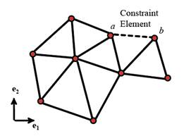
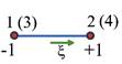
As a simple example, suppose that we wish to constrain two nodes a and b in a mesh to have the same displacement.   In this case the element connects nodes a and b, as shown in the figure.  The constraint equation is simply

$g=u_i^a-u_i^b$

For a two-dimensional mesh, we could choose to order the element degrees of freedom as $u^{el}=\left[u_1^a,u_2^a,u_1^b,u_2^b\right]$, in which case the stiffness and force are simply

$\begin{array}{l}{r}_{el}=G{\left[\begin{array}{cccc}{u}_1^a-u_1^b& u_2^a-u_2^b& -(u_1^a-u_1^b)& -(u_2^a-u_2^b)\end{array}\right]}^T\\ k_{el}=\left[\begin{array}{cccc}G& 0& -G& 0\\ 0& G& 0& -G\\ -G& 0& G& 0\\ 0& -G& 0& G\end{array}\right]\end{array}$

 

The penalty method is simple to implement, can be added to any standard FEA equations, and can be used in both static and dynamic analyses.   It has two drawbacks: (i) the constraint is not satisfied exactly, and (ii) the penalty coefficient G has to be chosen carefully: if G is too small, the constraint will not be satisfied, and if it is too large, it will make the stiffness matrix poorly conditioned, or make the stable time step in an explicit dynamic simulation very small.  G is usually chosen by trial and error: start with some rough guess, then check and see if the constraint is violated too severely.   If so, G must be increased (try increasing it by a factor of 10).  If the constraint is satisfied it may be possible to reduce G.   A more sophisticated approach is to estimate the magnitude of the stiffness matrix before the constraint is applied (e.g. find the average value of its diagonal), and then choose G to be some multiple (eg. 10⁴) of the stiffness measure. 

 

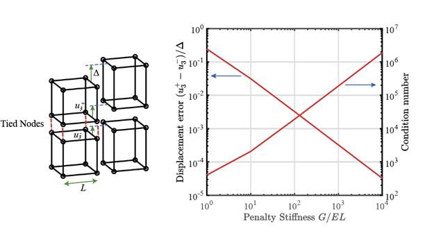
A simple illustration of a penalty element in action is shown in the figure.  The mesh consists of two separate hexahedral elements, as shown on the left.   Penalty elements are used to constrain the degrees of freedom on the four lower nodes of the top element to be equal to those on the four nodes on the top face of the bottom element.    The base of the lower element is prevented from moving vertically, while a prescribed vertical displacement $\Delta$ is applied to the top face of the upper element.   The graph plots the variation of the error in the constraint and the condition number of the global stiffness matrix as a function of the normalized penalty stiffness.   For low values of $G/L$ the matrix has a low condition number but the constraint is not enforced accurately; as $G/L$ increases the error diminishes, at the cost of an increase in the condition number.

 

A code that runs the test in this example is provided in the file FEM_Penaltyconstraint.m (along with input file Tie_constraint_example.txt) at

https://github.com/albower/Applied_Mechanics_of_Solids/

 

 

Enforcing constraints with a Lagrange Multiplier in static or implicit dynamic computations: There is a second, more sophisticated, way to enforce constraints.   The basic idea is simple: in the previous section the constraint was satisfied approximately by applying forces to the constrained nodes in the mesh. The forces were proportional to the deviation from the constraint, analogous to a linear spring.  Lagrange multipliers are reaction forces that enforce the constraint exactly.       

 

As before, we start by re-arranging the constraint equations into the form

$g^{(k)}(u_i^a)=0$

where a is the index of the M nodes; and k is an index identifying one of the constraint equations.  Each constraint is assigned an unknown reaction force (the Lagrange multiplier) ${\lambda }_k$, which must be determined along with the unknown displacements.    In addition, the work done by the reaction force must be added to the virtual work equation, which (using the VWE for a hypoelastic solid as a representative example) now takes the form

${\displaystyle \underset{R}{\int }{\sigma }_{ij}\left[{\epsilon }_{kl}(u_i^a)\right]{\displaystyle \frac{\partial N^a}{\partial x_j}dV+{\displaystyle \frac{\partial g^{(k)}}{\partial u_i^a}{\lambda }_k-{\displaystyle \underset{R}{\int }{b}_i{N}^{a}dV-{\displaystyle \underset{\partial R}{\int }{t}_i^{*}{N}^{a}dA}}}}}=0$

The unknown Lagrange multipliers are found by including the constraint equations in the global system.

 

The virtual work equation and the constraint equations are solved concurrently for the unknown displacements and Lagrange multipliers using Newton-Raphson iteration.  Since we need to solve for both displacements and Lagrange multipliers, the iteration proceeds by repeatedly solving a set of linear equations

$\begin{array}{l}{K}_{aibk}d{w}_k^b+{\displaystyle \frac{{\partial }^2{g}^{(m)}}{\partial u_i^a\partial u_k^b}{\lambda }_{m}d{w}_k^b+{\displaystyle \frac{\partial g^{(m)}}{\partial u_i^a}d{\omega }_m+R_i^a+{\displaystyle \frac{\partial g^{(m)}}{\partial u_i^a}{\lambda }_m-F_i^a=0}}}\\ {\displaystyle \frac{\partial g^{(m)}}{\partial u_k^b}d{w}_k^b+g^{(m)}=0}\end{array}$

for corrections $d{w}_i^a$ to the current approximation for the displacement field and corrections $d{\omega }_k$ to the Lagrange multipliers. The additional contributions to the equation system from the constraints are shown explicitly, and as usual

$K_{aibk}={\displaystyle \underset{R}{\int }{\displaystyle \frac{\partial {\sigma }_{ij}}{\partial {\epsilon }_{kl}}{\displaystyle \frac{\partial N^a}{\partial x_j}{\displaystyle \frac{\partial N^b}{\partial x_l}dV}}}}{R}_i^a={\displaystyle \underset{R}{\int }{\sigma }_{ij}\left[{\epsilon }_{kl}(w_i^b)\right]{\displaystyle \frac{\partial N^a}{\partial x_j}dV}}$

 

The extra terms from the constraints look scary, but it turns out that Lagrange multipliers can be added very easily to a standard static FEA code.   We simply create a new element for each constraint.   The element connects all the nodes in the constraint, and has one extra node, which has the Lagrange multiplier as an unknown degree of freedom.   The stiffness matrix and force vector for the constraint element are

$\begin{array}{l}{r}_{el}={\left[\begin{array}{ccccc}{\displaystyle \frac{\partial g^{(m)}}{\partial u_1^1}{\lambda }_m}& {\displaystyle \frac{\partial g^{(m)}}{\partial u_2^1}{\lambda }_m}& {\displaystyle \frac{\partial g^{(m)}}{\partial u_1^2}{\lambda }_m}& \cdots & g^{(m)}\end{array}\right]}^T\\ k_{el}=\left[\begin{array}{ccccc}{\displaystyle \frac{{\partial }^2{g}^{(m)}}{\partial u_1^1\partial u_1^1}{\lambda }_m}& {\displaystyle \frac{{\partial }^2{g}^{(m)}}{\partial u_1^1\partial u_2^1}{\lambda }_m}& {\displaystyle \frac{{\partial }^2{g}^{(m)}}{\partial u_1^1\partial u_1^2}{\lambda }_m}& \cdots & {\displaystyle \frac{\partial g^{(m)}}{\partial u_1^1}}\\ {\displaystyle \frac{{\partial }^2{g}^{(m)}}{\partial u_2^1\partial u_1^1}{\lambda }_m}& {\displaystyle \frac{{\partial }^2{g}^{(m)}}{\partial u_2^1\partial u_2^1}{\lambda }_m}& & & {\displaystyle \frac{\partial g^{(m)}}{\partial u_2^1}}\\ {\displaystyle \frac{{\partial }^2{g}^{(m)}}{\partial u_1^2\partial u_1^1}{\lambda }_m}& {\displaystyle \frac{{\partial }^2{g}^{(m)}}{\partial u_1^2\partial u_2^1}{\lambda }_m}& & & {\displaystyle \frac{\partial g^{(m)}}{\partial u_1^2}}\\ ⋮& & & & ⋮\\ {\displaystyle \frac{\partial g^{(m)}}{\partial u_1^1}}& {\displaystyle \frac{\partial g^{(m)}}{\partial u_2^1}}& {\displaystyle \frac{\partial g^{(m)}}{\partial u_1^2}}& \cdots & 0\end{array}\right]\end{array}$

 

 

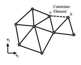
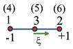
As a simple example, suppose that we wish to constrain two nodes a and b in a two-dimensional mesh to have the same displacement in the $e_1$ direction.   In this case the element connects nodes a and b, as shown in the figure.  The constraint equation is simply

$g=u_1^a-u_1^b$

For a 2D mesh, we could choose to order the element degrees of freedom as $u^{el}=\left[u_1^a,u_2^a,u_1^b,u_2^b,\lambda \right]$, in which case the stiffness and force are

$\begin{array}{l}{r}_{el}={\left[\begin{array}{ccccc}\lambda & 0& -\lambda & 0& u_1^a-u_1^b\end{array}\right]}^T\\ k_{el}=\left[\begin{array}{ccccc}0& 0& 0& 0& 1\\ 0& 0& 0& 0& 0\\ 0& 0& 0& 0& -1\\ 0& 0& 0& 0& 0\\ 1& 0& -1& 0& 0\end{array}\right]\end{array}$

 

It may seem odd to include both components of displacement for the nodes in the vector of element degrees of freedom: this is not essential, but makes it easier to add the contribution from the Lagrange multiplier element to the global equation system.  If (as in the preceding section) we wish to force nodes a and b to have the same displacement in all directions, we simply create a separate Lagrange multiplier element for each displacement component.

 

A final observation is helpful if you are thinking of using Lagrange multipliers in your code. Some old equation solvers which solve the finite element linear system of equations by Gaussian elimination without pivoting may have difficulties handling the zero diagonal that appears in the stiffness for the Lagrange multiplier degrees of freedom. Fortunately, this is rarely a problem with modern sparse equation solvers.

 

A code that implements Lagrange multipliers is provided in the file FEM_LagrangeMultiplierconstraint.m (along with input file Tie_constraint_example.txt) at

https://github.com/albower/Applied_Mechanics_of_Solids/

 

 

Enforcing constraints with a Lagrange Multiplier in explicit dynamic computations. Explicit dynamic computations were described in Section 8.2.4 (for the special case of a linear elastic solid).  More generally, they are an efficient way to solve equations of motion of the form

$M_{ab}{\ddot{u}}_i^b+R_i^a=F_i^a$

where (for small strains, but nonlinear material behavior)

$R_i^b={\displaystyle \underset{R}{\int }{\sigma }_{ij}\left[u_k^b\right]{\displaystyle \frac{\partial N^a}{\partial x_j}dV}}{F}_i^a={\displaystyle \underset{R}{\int }{b}_i{N}^{a}dV+{\displaystyle \underset{\partial R}{\int }{t}_i^{*}{N}^{a}dA}}$

are the internal and external force vectors, and $M_{ab}$ is the diagonal ‘lumped’ mass matrix for a finite element mesh.   Without constraints, this equation is usually solved using the explicit dynamic version of the more general ‘Newmark’ time integration scheme described in Section 8.2.4.  This works as follows: we are given the initial nodal velocities $v_i^a(0)$ and displacements $u_i^a(0)$.  The time-stepping starts by computing (at time t=0) the initial acceleration

$a_i^a(0)=M_{ab}^{-1}\left[-R_i^b\left(u_i^a(0)\right)+F_i^b(0)\right]$,

Then, for successive time steps

 

1. Calculate the displacements at time $t+\Delta t$ as

$u_i^a(t+\Delta t)\approx u_i^a(t)+\Delta t{\dot{u}}_i^a(t)+{\displaystyle \frac{\Delta t^2}{2}{a}_i^a(t)}$

 

2. Calculate the accelerations at time $t+\Delta t$

$a_i^a(t+\Delta t)=M_{ab}^{-1}\left[-R_i^b\left(u_i^a(t+\Delta t)\right)+F_i^b(t+\Delta t)\right]$

Recall that M is diagonal, so the equation solving is trivial: this is the main advantage of explicit dynamics.

 

3. Update the velocity as

$v_i^a(t+\Delta t)\approx v_i^a(t)+{\displaystyle \frac{\Delta t}{2}\left[a_i^a(t)+a_i^a(t+\Delta t)\right]}$

 

 

We now wish to solve a modified problem in which some subset of nodes is constrained by equations of the form

$g^{(k)}(u_i^a)=0$

(the initial displacements must satisfy the constraints).   It is not possible to enforce this type of constraint using Lagrange multipliers in the standard explicit dynamic Newmark algorithm, because the Lagrange multipliers have no mass.   Instead, a two-step ‘predictor-corrector’ method  is used for this purpose, as follows.   The procedure begins by calculating the initial accelerations $a_i^a(0)$ using the usual expressions.  Then, for successive time steps:

 

1. Predictor step: Compute predictors for the accelerations, velocity and displacement $\overline{a}(t+\Delta t),\overline{v}(t+\Delta t),\overline{u}(t+\Delta t)$ (without enforcing constraints) using the standard Newmark procedure:

$u_i^a(t+\Delta t)\approx u_i^a(t)+\Delta t{\dot{u}}_i^a(t)+{\displaystyle \frac{\Delta t^2}{2}{a}_i^a(t)}$

${\overline{a}}_i^a(t+\Delta t)=M_{ab}^{-1}\left[-R_i^b\left(u_i^a(t+\Delta t)\right)+F_i^b(t+\Delta t)\right]$

${\overline{v}}_i^a(t+\Delta t)\approx v_i^a(t)+{\displaystyle \frac{\Delta t}{2}\left[a_i^a(t)+{\overline{a}}_i^a(t+\Delta t)\right]}$

${\overline{u}}_i^a(t+\Delta t)\approx u_i^a(t)+\Delta t{\overline{v}}_i^a(t+\Delta t)+{\displaystyle \frac{\Delta t^2}{2}{\overline{a}}_i^a(t+\Delta t)}$

 

2. Corrector step: Calculate the correct accelerations for each constrained node, along with the Lagrange multiplier for the constraint, by solving the following system of linear equations

$\begin{array}{l}{M}_{ab}{a}_i^b(t+\Delta t)+{\displaystyle \frac{\partial g^{(m)}}{\partial u_i^a}{\lambda }_m=M_{ab}{\overline{a}}_i^b(t+\Delta t)}\\ {\displaystyle \frac{\partial g^{(m)}}{\partial u_k^b}{a}_k^b(t+\Delta t)=-{\displaystyle \frac{1}{\Delta t^2}{g}^{(m)}\left(u_i^a(t)\right)-{\displaystyle \frac{\partial g^{(m)}}{\partial u_k^b}\left({\displaystyle \frac{1}{\Delta t}{v}_k^b(t)+{\displaystyle \frac{1}{2}{a}_k^b(t)}}\right)}}}\end{array}$

and then, update the velocity and displacement for the constrained nodes using the standard Newmark algorithm with the corrected accelerations

$v_i^a(t+\Delta t)\approx v_i^a(t)+{\displaystyle \frac{\Delta t}{2}\left[a_i^a(t)+a_i^a(t+\Delta t)\right]}$

${\overline{u}}_i^a(t+\Delta t)\approx u_i^a(t)+\Delta t{v}_i^a(t+\Delta t)+{\displaystyle \frac{\Delta t^2}{2}{a}_i^a(t+\Delta t)}$

 

For example, to constrain two nodes a and b in a two-dimensional mesh to have the same displacement in the $e_1$ direction.   The constraint equation is then

$g=u_1^a-u_1^b$

The equation system for the corrector step is then

 

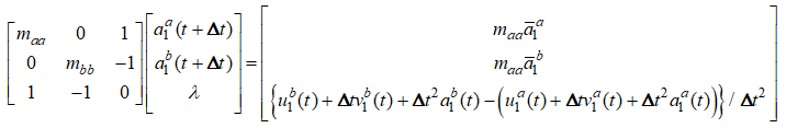
where $m_{aa},m_{bb}$ are the lumped masses of nodes a and b. Notice that if all constraints are ties between two degrees of freedom, they may be treated independently.  This requires only a solution of a 3x3 linear system for each tie at each time-step, which can be done quickly.

 

The predictor-corrector algorithm can be derived as follows.    The constrained equation system (with the correct accelerations) has the form

$\begin{array}{l}{M}_{ab}{a}_i^b+R_i^a+{\displaystyle \frac{\partial g^{(m)}}{\partial u_i^a}{\lambda }_m=F_i^a}\\ g^{(k)}(u_i^a)=0\end{array}$

The predictor accelerations neglect the constraints, and therefore satisfy

$M_{ab}{\overline{a}}_i^b+R_i^a=F_i^a$

Subtracting this from the constrained equation system yields

$\begin{array}{l}{M}_{ab}(a_i^b-{\overline{a}}_i^b)+{\displaystyle \frac{\partial g^{(m)}}{\partial u_i^a}{\lambda }_m=0}\\ g^{(k)}(u_i^a)=0\end{array}$

We satisfy this equation at the end of the time-step, using the standard Newmark approximation for the displacement

$u_i^a(t+\Delta t)\approx u_i^a(t)+\Delta t{v}_i^a(t+\Delta t)+{\displaystyle \frac{\Delta t^2}{2}{a}_i^a(t+\Delta t)}$

Substituting this expression for the displacements and expanding the constraint equation for small $\Delta t$ then yields

$\begin{array}{l}{M}_{ab}{a}_i^b(t+\Delta t)+{\displaystyle \frac{\partial g^{(m)}}{\partial u_i^a}{\lambda }_m=M_{ab}{\overline{a}}_i^b(t+\Delta t)}\\ g^{(m)}\left(u_i^a(t)\right)+{\displaystyle \frac{\partial g^{(m)}}{\partial u_k^b}\left(\Delta t{v}_k^b(t)+{\displaystyle \frac{\Delta t^2}{2}{a}_k^b(t)+\Delta t^2{a}_k^b(t+\Delta t)}\right)=0}\end{array}$

This can be rearranged into the equation system for the corrector step.

 

In practice, explicit dynamic simulations tend to enforce constraints with the penalty method rather than Lagrange multipliers, because solving for the Lagrange multipliers can slow down the explicit dynamic Newmark algorithm.   The two exceptions are simple tie constraints, which can be enforced without solving large systems of equations, and handling ‘hard’ contact between two solids, where it is preferable to enforce the constraints between contacting nodes and elements exactly.   

 

A code that implements this algorithm is provided in the file FEM_dynamic_constraints.m (along with input file dynamic_constrained_beam.txt) at

https://github.com/albower/Applied_Mechanics_of_Solids/

 

The code animates a vibrating beam, which has a single element connected to its end by Lagrange multiplier constraints.

 

 

 

8.8.2 Modeling interface fracture: Cohesive zone elements

 

Cohesive zones are used to model the nucleation and propagation of cracks along weak interfaces in a solid, as well as to model adhesion between two contacting surfaces.   They are described in detail in Section 3.13.1.   Here, we describe how a cohesive zone can be added to a finite element simulation. To keep things simple, we describe a small displacement cohesive zone element.

 

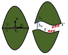Example traction-separation law for cohesive interfaces: The figure shows a representative interface between two solids before and after it separates.   The displacement and forces acting on the two surfaces adjacent to the interface are quantified as follows:

 

1. Introduce a basis $\{n,e_1,e_2\}$ with $e_{\alpha }$ in the plane of the interface and $n$ normal to it.   The vector n can point in either direction perpendicular to the interface, but once chosen, we designate the surface with normal n as $S^{-}$ and that with normal -n as $S^{+}$.

 

2. The relative displacement of two points on $S^{-},S^{+}$ that are coincident in the undeformed solid $\Delta =u^{+}-u^{-}$, and has components $\left\{\Delta {}_n,{\Delta }_1,{\Delta }_2\right\}$ in $\{n,e_1,e_2\}$.  The tangential component of displacement is ${\Delta }_t=\sqrt{{\Delta }_1^2+{\Delta }_2^2}$

 

3. The tractions on the two adjacent surfaces are quantified by the traction components $\{T_1,T_2,T_n\}$ acting on $S^{-}$.

 

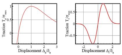
Constitutive equations for a cohesive interface relate $\left\{{\Delta }_1,{\Delta }_2,{\Delta }_n\right\}$ and $\{T_1,T_2,T_n\}$.  To keep things simple, in this section we implement a finite element solution for a widely used cohesive zone law originally developed by Xu and Needleman (1995).   The tractions are related to the displacements by:

$\begin{array}{l}{T}_{\alpha }=2{\sigma }_{\max }\left({\displaystyle \frac{{\Delta }_{\alpha }}{{\delta }_n}}\right)\left(1+{\displaystyle \frac{{\Delta }_n}{{\delta }_n}}\right)\exp \left(1-{\displaystyle \frac{{\Delta }_n}{{\delta }_n}}\right)\exp \left(-{\displaystyle \frac{{\Delta }_t^2}{{\delta }_n^2}}\right)+\eta {\displaystyle \frac{d{\Delta }_{\alpha }}{dt}}\\ T_n={\sigma }_{\max }{\displaystyle \frac{{\Delta }_n}{{\delta }_n}\exp \left(1-{\displaystyle \frac{{\Delta }_n}{{\delta }_n}}\right)\exp \left(-{\displaystyle \frac{{\Delta }_t^2}{{\delta }_n^2}}\right)+\eta {\displaystyle \frac{d{\Delta }_n}{dt}}}\end{array}$

where $({\sigma }_{\max },{\delta }_n,\eta )$ are material properties.   The parameter ${\sigma }_{\max }$ is the strength of the interface in tension; ${\delta }_n$ is the normal separation corresponding to the maximum stress; and $\eta$ is a small viscosity.  In the quasi-static limit the work of separation per unit area for the interface is $\varphi ={\sigma }_{\max }{\delta }_n\exp (1)$ per unit area.  The viscous term is sometimes omitted, but helps to ensure that sudden nucleation of a crack in the interface does not cause convergence problems during the Newton-Raphson solution of the equilibrium equations.  Usually, simulations are run with as small a viscosity as possible.    The variation of normal and tangential traction with normal and tangential relative displacement of the two solids adjacent to the interface is shown in the figure below.

 

 

 

Finite element equations: We account for the cohesive interface in a finite element simulation by adding the work done by the tractions acting on the two sides of the interface to the virtual work equation.   For example, the discrete virtual work equation for a hypoelastic solid becomes

${\displaystyle \underset{R}{\int }{\sigma }_{ij}\left[{\epsilon }_{kl}(u_i^a)\right]{\displaystyle \frac{\partial N^a}{\partial x_j}dV+{\displaystyle \underset{\Gamma }{\int }(T_n{n}_i+T_{\alpha }{e}_i^{(\alpha )})\left[N^{a+}-N^{a-}\right]}-{\displaystyle \underset{R}{\int }{b}_i{N}^{a}dV-{\displaystyle \underset{\partial R}{\int }{t}_i^{*}{N}^{a}dA}}}}=0$

where $(n_i,e_i^{(\alpha )})$ are the components of $(n,e_{\alpha })$ , $N^{a+}$, $N^{a-}$ denote the interpolation functions for the element faces connecting the nodes adjacent to  $S^{+}$ and $S^{-}$, and $\Gamma$ denotes the surface (or line) defining the interface.   The additional term can be added to any of the virtual work equations covered in Chapter 8.   Even if the solid is a linear elastic material, the virtual work equation is nonlinear, because the traction-separation law for the interface is nonlinear.  In addition, the traction-separation law is rate dependent, so the load must be applied in a series of time increments $\Delta t$, and at each step the increment of displacement $\Delta u_i^a$ must be found by Newton-Raphson iteration.  This means repeatedly solving a set of linear equations

$K_{aibk}d{w}_k^b+R_i^a-F_i^a=0$

for corrections $d{w}_i^a$ to the current approximation for the displacement increment, where the stiffness and internal force vector now include contributions from the interfaces

$\begin{array}{l}{K}_{aibk}={\displaystyle \underset{R}{\int }{\displaystyle \frac{\partial {\sigma }_{ij}}{\partial {\epsilon }_{kl}}{\displaystyle \frac{\partial N^a}{\partial x_j}{\displaystyle \frac{\partial N^b}{\partial x_l}dV}}}}\\ +{\displaystyle \underset{\Gamma }{\int }\left[N^{b+}-N^{b-}\right]\left((n_k{\displaystyle \frac{\partial T_n}{\partial {\Delta }_n}+e_k^{(\alpha )}{\displaystyle \frac{\partial T_n}{\partial {\Delta }_{\alpha }}{n}_i+e_k^{(\beta )}{\displaystyle \frac{\partial T_{\alpha }}{\partial {\Delta }_{\beta }}{e}_i^{(\alpha )}+n_k{\displaystyle \frac{\partial T_{\alpha }}{\partial {\Delta }_n}{e}_i^{(\alpha )})}}}}\right)\left[N^{a+}-N^{a-}\right]}\\ R_i^a={\displaystyle \underset{R}{\int }{\sigma }_{ij}\left[{\epsilon }_{kl}(w_i^b)\right]{\displaystyle \frac{\partial N^a}{\partial x_j}dV}}+{\displaystyle \underset{\Gamma }{\int }(T_n{n}_i+T_{\alpha }{e}_i^{(\alpha )})\left[N^{a+}-N^{a-}\right]dA}\end{array}$

The additional contributions to $K_{aibk}$ and $R_i^a$ from the interface can be added by meshing the interface with planar ‘cohesive zone’ elements.   To begin, the solids adjacent to the element are meshed in the usual way with standard continuum elements, but the meshes are designed so that (i) the same element geometry and interpolation scheme is used in both solids, and (ii) the two solids have coincident nodes on the interface.    The interface can then be meshed with planar triangular or quadrilateral elements (in 3D) or linear or quadratic line elements (in 2D).   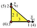The order of interpolation should be consistent with the solid elements adjacent to the interface.   Representative interface elements (with the nodes attached to the two solids shown separated for clarity) are shown in the figure below.

 

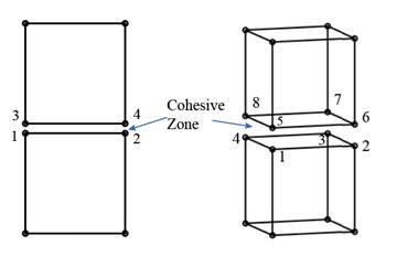
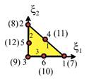
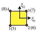
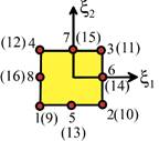
The displacement field is then interpolated within each element using the shape functions listed in the tables below, as follows.   The nodes on the interface element are numbered so that those on $S^{-}$ have the lowest node numbers.  For example, for a linear line element, nodes 1 and 2 lie on $S^{-}$, while nodes 3 and 4 are the nodes on $S^{+}$ that are coincident with nodes 1 and 2, respectively.   For a linear quadrilateral element, nodes 1-4 lie on $S^{-}$, and nodes 5-8 lie on $S^{+}$, with node 5 coincident with node 1 in the undeformed solid, and so on.

 

 

 

 

 

 

 

 

 

Taking an 8 noded linear cohesive zone element between two 8 noded hexahedral elements as a representative example, we then perform the following calculations for each integration point in the element:

 

1. Assemble the vector of nodal coordinates $x={\left[x_1^{(1)},x_2^{(1)},x_3^{(1)},x_1^{(1)}\cdots x_1^{(4)},x_2^{(4)},x_3^{(4)}\right]}^T$ and the 2D matrix of shape function derivatives

${\displaystyle \frac{dN}{d\xi }=\left[\begin{array}{cccc}{\displaystyle \frac{\partial N^1}{\partial {\xi }_1}}& {\displaystyle \frac{\partial N^2}{\partial {\xi }_1}}& {\displaystyle \frac{\partial N^3}{\partial {\xi }_1}}& {\displaystyle \frac{\partial N^4}{\partial {\xi }_1}}\\ {\displaystyle \frac{\partial N^1}{\partial {\xi }_2}}& {\displaystyle \frac{\partial N^2}{\partial {\xi }_2}}& {\displaystyle \frac{\partial N^3}{\partial {\xi }_2}}& {\displaystyle \frac{\partial N^4}{\partial {\xi }_2}}\end{array}\right]}$

where $N^a$ with a=1…4 are the interpolation functions for the 4 noded quadrilateral elements listed in Table 8.3 and hence calculate

$\begin{array}{l}{\displaystyle \frac{dx}{d\xi }=\left[\begin{array}{c}{\displaystyle \frac{dx}{d{\xi }_1}}\\ {\displaystyle \frac{dx}{d{\xi }_2}}\end{array}\right]={\displaystyle \frac{dN}{d\xi }xJ=\left|{\displaystyle \frac{dx}{d{\xi }_1}\times {\displaystyle \frac{dx}{d{\xi }_2}}}\right|}}\\ n={\displaystyle \frac{1}{J}{\displaystyle \frac{dx}{d{\xi }_1}\times {\displaystyle \frac{dx}{d{\xi }_2}{e}_1={\displaystyle \frac{1}{\left|dx/d{\xi }_1\right|}{\displaystyle \frac{dx}{d{\xi }_1}{e}_2=n\times e_1}}}}}\end{array}$

 

2. Assemble a matrix B that maps displacement components in the $\{i,j,k\}$ directions to the normal and tangential displacement jump at an arbitrary point in the element by defining (for a 3D element)

${\left[{\Delta }_n,{\Delta }_1,{\Delta }_2\right]}^T=B{\left[\begin{array}{ccccc}{u}_1^1& u_2^1& u_3^1& u_1^2& \cdots \end{array}\right]}^T$

For a linear 8 noded quadrilateral cohesive zone element the B matrix is

 

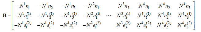
where $(n_i,e_i^{(\alpha )})$ are the components of $(n,e_{\alpha })$.  Similar matrices can be constructed for other elements using the definition.

 

3. Calculate the displacement jumps $\left[{\Delta }_n,{\Delta }_1,{\Delta }_2\right]$, determine the time derivative of the displacement jumps by dividing the increment in displacement by the time increment, and hence use the traction-separation law to assemble the traction vector $T={\left[T_n,T_1,T_2\right]}^T$.

 

4. Assemble a tangent matrix D that quantifies the stiffness of the interface.  For a 3D interface

$D=\left[\begin{array}{ccc}{\displaystyle \frac{\partial T_n}{\partial {\Delta }_n}}& {\displaystyle \frac{\partial T_n}{\partial {\Delta }_1}}& {\displaystyle \frac{\partial T_n}{\partial {\Delta }_2}}\\ {\displaystyle \frac{\partial T_1}{\partial {\Delta }_n}}& {\displaystyle \frac{\partial T_1}{\partial {\Delta }_1}}& {\displaystyle \frac{\partial T_1}{\partial {\Delta }_2}}\\ {\displaystyle \frac{\partial T_2}{\partial {\Delta }_n}}& {\displaystyle \frac{\partial T_2}{\partial {\Delta }_1}}& {\displaystyle \frac{\partial T_2}{\partial {\Delta }_2}}\end{array}\right]$

The derivatives in this matrix are

$\begin{array}{l}{\displaystyle \frac{\partial T_n}{\partial {\Delta }_n}={\displaystyle \frac{{\sigma }_{\max }}{{\delta }_n}\left(1-{\displaystyle \frac{{\Delta }_n}{{\delta }_n}}\right)\exp \left(1-{\displaystyle \frac{{\Delta }_n}{{\delta }_n}}\right)\exp \left(-{\displaystyle \frac{{\Delta }_t^2}{{\delta }_n^2}}\right)+{\displaystyle \frac{\eta }{\Delta t}}}}\\ {\displaystyle \frac{\partial T_n}{\partial {\Delta }_{\alpha }}={\displaystyle \frac{\partial T_{\alpha }}{\partial {\Delta }_n}=-2{\displaystyle \frac{{\sigma }_{\max }}{{\delta }_n}{\displaystyle \frac{{\Delta }_n{\Delta }_{\alpha }}{{\delta }_n^2}\exp \left(1-{\displaystyle \frac{{\Delta }_n}{{\delta }_n}}\right)\exp \left(-{\displaystyle \frac{{\Delta }_t^2}{{\delta }_n^2}}\right)}}}}\\ {\displaystyle \frac{\partial T_{\alpha }}{\partial {\Delta }_{\beta }}=2{\displaystyle \frac{{\sigma }_{\max }}{{\delta }_n}\left({\delta }_{\alpha \beta }-2{\displaystyle \frac{{\Delta }_{\alpha }{\Delta }_{\beta }}{{\delta }_n^2}}\right)\left(1+{\displaystyle \frac{{\Delta }_n}{{\delta }_n}}\right)\exp \left(1-{\displaystyle \frac{{\Delta }_n}{{\delta }_n}}\right)\exp \left(-{\displaystyle \frac{{\Delta }_t^2}{{\delta }_n^2}}\right)+{\displaystyle \frac{\eta }{\Delta t}{\delta }_{\alpha \beta }}}}\end{array}$

 

 

The element stiffness and internal force vector for the cohesive zone element can then be calculated as

$k_{el}={\displaystyle \sum _i{B}^T({\xi }_i)D({\xi }_i)B({\xi }_i)J({\xi }_i)w_i}{r}_{el}={\displaystyle \sum _i{B}^T({\xi }_i)T({\xi }_i)J({\xi }_i)w_i}$

where ${\xi }_i,w_i$ are the integration points and weights for a 2x2 point Gaussian quadrature scheme (see Section 8.1.12).

 

 

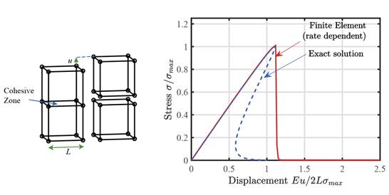
Example: A simple example of the use of a cohesive zone element to predict interface separation is shown in the figure. Two solid cubes with side length L (meshed with a single element) are bonded by a cohesive interface.  Both cubes have the same Young’s modulus E.  The interface has strength ${\sigma }_{\max }$, separation ${\delta }_n$ at peak stress; and viscosity $\eta$.  The bottom cube is prevented from displacing vertically, and the top face of the upper cube is displaced vertically by distance u(t) at constant rate $V_0$.  The cubes are in a state of uniaxial vertical stress with magnitude $\sigma$.   The graph shows the stress in the cubes as a function of the imposed displacement.   For comparison, the exact solution for a rate independent interface can be expressed in parametric form as

${\displaystyle \frac{\sigma }{{\sigma }_{\max }}={\displaystyle \frac{\delta }{{\delta }_n}\exp \left(1-{\displaystyle \frac{\delta }{{\delta }_n}}\right){\displaystyle \frac{Eu}{2L{\sigma }_{\max }}={\displaystyle \frac{\delta }{{\delta }_n}\left\{{\displaystyle \frac{E{\delta }_n}{L{\sigma }_{\max }}+\exp \left(1-{\displaystyle \frac{\delta }{{\delta }_n}}\right)}\right\}}}}}$

The result is plotted as a dashed curve in the figure.   Results are shown for $E{\delta }_n/(2L{\sigma }_{\max })=0.1$ and $\eta V_0/{\sigma }_{\max }=0.0025$.  The interface experiences a ‘snap back’ instability, in which the stress-displacement relation for the rate-independent interface has a portion with negative slope.   Since a monotonically increasing displacement is prescribed on the upper solid in the finite element simulation, the interface experiences a rapid separation (at a rate determined by the viscosity of the interface) and the stress drops rapidly from a value close to its peak to close to zero.   If the simulation is attempted with $\eta =0$, the Newton-Raphson equilibrium iterations fail to converge at the point where the instability occurs, and the simulation terminates.

 

A code that runs the test in this example is provided in the file FEM_Cohesive_Zones.m (along with input files CohesiveZone_example.txt and CohesiveZone_Example_2D) at

https://github.com/albower/Applied_Mechanics_of_Solids/

 

 

 

8.8.3 Modeling Contact

 

We end this chapter with a brief description how contact between two deformable solids can be treated in a finite element simulation.   To keep things simple we consider only two-dimensional, static, ‘hard’ frictionless contact, but we will account for large changes in the geometry of the contacting solids.

 

Contact geometry:  The figure shows the problem to be solved.  We anticipate that two finite element meshes may come into contact during an analysis (or the mesh may contact itself).   Wherever contact does occur, we must prevent the meshes from overlapping.   We therefore need a way to calculate the gap between the two surfaces.

 

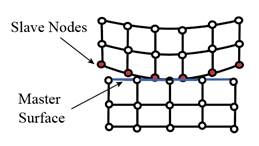
To do this, we designate one of the contacting surfaces as the ‘master,’ and the other as ‘slave.’   The choice is arbitrary, but it can be helpful to select the stiffer of the two surfaces as the ‘master.’   We then fit a curve through the nodes on the master surface in some way: this curve is used to define the boundary of the solid.  Here, we will connect the nodes with straight-line segments, but quadratic or higher order polynomials are often used as well.  The contact algorithm must prevent the nodes on the ‘slave’ surface from penetrating within the ‘master’ curve.

 

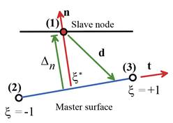A representative slave node (given the number 1) and master segment (connecting nodes 2 and 3) is shown in the figure. The nodes have positions (after deformation) $y^a$, a=1..3.   For subsequent calculations it is helpful to define a set of interpolation functions that will be used to calculate the gap between the node 1 and the master segment:

$\begin{array}{l}{N}^1=-1N^2=(1-\xi )/2\\ N^3=(1+\xi )/2-1<\xi <1\end{array}$

It is helpful to note that

 

1. a vector from the slave node to a point at normalized coordinate $\xi$ on the master segment can be calculated as $d=N^a(\xi )y^a$. 

 

2. A unit vector tangent to the master surface can be calculated as

$t={\displaystyle \frac{1}{\left|(\partial N^a/\partial \xi )y^a\right|}{\displaystyle \frac{\partial N^a}{\partial \xi }{y}^a}}$

 

3. A unit vector normal to the master surface follows as $n=[-t_2,t_1]$

 

In addition, the calculations described here can be extended to a curved geometry for the master segment by including more master nodes, and interpolating between their positions using higher order polynomials for $N^a$.

 

The gap between the slave node and the master segment is then calculated as follows:

1. Determine the point ${\xi }^{*}$ on the master segment that is closest to the slave node from the condition $d({\xi }^{*})\cdot t=0$.   For a straight line master segment this is a linear equation with solution

${\xi }^{*}=\left(y^3-y^2\right)\cdot \left(2y^1-y^2-y^3\right)/{\left|y^3-y^2\right|}^2$

For higher order master segments the equation is nonlinear and must be solved numerically.

 

2. Calculate the gap from ${\Delta }_n=-n\cdot N^a({\xi }^{*})y^a$.

 

The finite element solution must then satisfy: (i) ${\Delta }_n\ge 0$ for all slave nodes and (ii) The reaction force between master surface and slave node must be repulsive or zero.   In a static analysis, these conditions are satisfied by iteration, as follows:

 

1.       Start with some guess for the nodes that are in contact;

 

2.       Solve the equilibrium equation while enforcing the condition ${\Delta }_n=0$ for these nodes

 

3.       Calculate ${\Delta }_n$ for slave nodes that were not included in the contact set, and add any with ${\Delta }_n<0$ to the contact set for the next iteration

 

4.       Calculate the reaction force for slave nodes in the contact set and remove any with tensile reactions from the contact set for the next iteration

 

5.       Check that $-1<{\xi }^{*}<1$ for all slave nodes.   If not, a slave node has slid from one master segment to its neighbor.    Update the connectivity for the master-slave elements for the next iteration.

 

6.       If there was a change in the list of contacting nodes or the master-slave connectivity, return to step 2.

 

 

Constrained virtual work equation: The constraints at slave nodes are satisfied using Lagrange multipliers, as described in Section 8.8.1. Using the hypoelastic solid as a representative example again, the modified virtual work equation takes the form

${\displaystyle \underset{R}{\int }{\sigma }_{ij}\left[{\epsilon }_{kl}(u_i^a)\right]{\displaystyle \frac{\partial N^a}{\partial x_j}dV+{\displaystyle \frac{\partial {\Delta }_n{}^{(c)}}{\partial u_i^a}{\lambda }_c-{\displaystyle \underset{R}{\int }{b}_i{N}^{a}dV-{\displaystyle \underset{\partial R}{\int }{t}_i^{*}{N}^{a}dA}}}}}=0$

where a summation on slave nodes c is implied, and

${\displaystyle \frac{\partial {\Delta }_n}{\partial u_i^a}=-N^a({\xi }^{*})n_i}$

As usual the discrete virtual work equation is a set of nonlinear equations for the unknown displacements $u_i^a$ at the nodes.  The additional unknown Lagrange multipliers are found by including the constraint equations ${\Delta }_n^{(c)}$ at the contacting slave nodes in the global system.   The equations must be solved using Newton-Raphson iterations, which means repeatedly solving a set of linear equations

$\begin{array}{l}{K}_{aibk}d{w}_k^b+{\displaystyle \frac{{\partial }^2{\Delta }_n^{(c)}}{\partial u_i^a\partial u_k^b}{\lambda }_{c}d{w}_k^b+{\displaystyle \frac{\partial {\Delta }_n^{(c)}}{\partial u_i^a}d{\omega }_c+R_i^a+{\displaystyle \frac{\partial {\Delta }_n^{(c)}}{\partial u_i^a}{\lambda }_c-F_i^a=0}}}\\ {\displaystyle \frac{\partial {\Delta }_n^{(c)}}{\partial u_k^b}d{w}_k^c+{\Delta }_n^{(c)}=0}\end{array}$

for corrections $d{w}_i^a$ to the current approximation for the displacement field and corrections $d{\omega }_k$ to the Lagrange multipliers. As usual

$K_{aibk}={\displaystyle \underset{R}{\int }{\displaystyle \frac{\partial {\sigma }_{ij}}{\partial {\epsilon }_{kl}}{\displaystyle \frac{\partial N^a}{\partial x_j}{\displaystyle \frac{\partial N^b}{\partial x_l}dV}}}}{R}_i^a={\displaystyle \underset{R}{\int }{\sigma }_{ij}\left[{\epsilon }_{kl}(w_i^b)\right]{\displaystyle \frac{\partial N^a}{\partial x_j}dV}}$

while

${\displaystyle \frac{{\partial }^2{\Delta }_n^{(c)}}{\partial u_i^a\partial u_k^b}\approx -p{\displaystyle \frac{N^a{N}^b}{q^2}{t}_k{t}_i+{\displaystyle \frac{N^a}{q}{\displaystyle \frac{\partial N^b}{\partial \xi }{t}_i{n}_k+{\displaystyle \frac{N^b}{q}{\displaystyle \frac{\partial N^a}{\partial \xi }{t}_k{n}_i}}}}}}$

with

$q=\left|{\displaystyle \frac{\partial N^a}{\partial \xi }{y}^a}\right|p=n\cdot {\displaystyle \frac{{\partial }^2{N}^a}{\partial {\xi }^2}{y}^a}$

For a straight-line master segment p=0.

 

The derivatives of ${\Delta }_n^{(c)}$ in these expressions are derived as follows:

1. Recall that ${\Delta }_{n}n=-N^a{y}^a$.  

 

2. Perturbing this expression shows that

$\delta {\Delta }_{n}n+{\Delta }_n\delta n=-N^a\delta y^a-{\displaystyle \frac{\partial N^a}{\partial \xi }\delta {\xi }^{*}{y}^a}$

 

3. The second term on both the left and right hand sides of this expression must be parallel to the tangent vector t.  If we dot both sides with n, therefore, $\delta {\Delta }_n=-N^{a}n\cdot \delta y^a$. This shows that

${\displaystyle \frac{\partial {\Delta }_n}{\partial u_i^a}=-N^a({\xi }^{*})n_i}$

as required.

 

4. As an expedient approximation we can also assume ${\Delta }_n\approx 0$ in step (2), so taking the dot product of both sides with t shows that

$0=-N^{a}t\cdot \delta y^a-t\cdot {\displaystyle \frac{\partial N^a}{\partial \xi }{y}^a\delta {\xi }^{*}=-N^{a}t\cdot \delta y^a-q\delta {\xi }^{*}}$

We therefore see that

${\displaystyle \frac{\partial {\xi }^{*}}{\partial u_k^b}=-{\displaystyle \frac{N^b}{q}{t}_k}}$

 

5. Since $n\cdot t=0$ it follows that $t\cdot \delta n=-n\cdot \delta t$.   Recalling that $qt={\displaystyle \frac{\partial N^a}{\partial \xi }{y}^a}$, we see that

$q\delta t+\delta qt={\displaystyle \frac{{\partial }^2{N}^a}{\partial {\xi }^2}{y}^a\delta {\xi }^{*}+{\displaystyle \frac{\partial N^a}{\partial \xi }\delta y^a}}$

so that

$qt\cdot \delta n=-qn\cdot \delta t=-n\cdot {\displaystyle \frac{{\partial }^2{N}^a}{\partial {\xi }^2}{y}^a\delta {\xi }^{*}-{\displaystyle \frac{\partial N^a}{\partial \xi }n\cdot \delta y^a=-p\delta {\xi }^{*}-{\displaystyle \frac{\partial N^a}{\partial \xi }n\cdot \delta y^a}}}$

 

6. Noting that $\delta n$ is parallel to t and using the result of (4) then shows that

${\displaystyle \frac{\partial n_i}{\partial u_k^b}={\displaystyle \frac{p}{q^2}{N}^b{t}_i{t}_k-{\displaystyle \frac{\partial N^b}{\partial \xi }{t}_i{n}_k}}}$

Finally, differentiating (3) and using (4) and (6) gives the required second derivative of ${\Delta }_n$

 

As usual the virtual work equation looks confusing in index notation, but the expressions for the stiffness matrix and residual force vector look simpler when expressed in matrix form.   We create a single contact element for each slave node, which also is attached to two (for a linear master segment) nodes on the master surface, as well as a Lagrange multiplier node with a single degree of freedom.  The residual force vector and stiffness for this element are assembled into the global system of equations in the usual way. The degrees of freedom for the contact element can be ordered as $\left[u_1^1,u_2^1,u_1^2,\cdots \lambda \right]$, in which case the element residual force vector and stiffness matrix have the form:

$r_{el}=\left[\begin{array}{ccccccc}-\lambda N^1{n}_1& -\lambda N^1{n}_2& -\lambda N^2{n}_1& -\lambda N^2{n}_2& -\lambda N^3{n}_1& -\lambda N^3{n}_2& {\Delta }_n\end{array}\right]$

$k_{el}={\displaystyle \frac{\lambda }{q}\left(\mu \otimes \tau +\tau \otimes \mu \right)-{\displaystyle \frac{\lambda p}{q^2}\tau \otimes \tau -\omega \otimes \nu -\nu \otimes \omega }}$

where $a\otimes b\equiv a_i{b}_j$ denotes an outer product, and

$\begin{array}{l}\tau =\left[\begin{array}{ccccccc}{N}^1{t}_1& N^1{t}_2& N^2{t}_1& N^2{t}_2& N^3{t}_1& N^3{t}_2& 0\end{array}\right]\\ \nu =\left[\begin{array}{ccccccc}{N}^1{n}_1& N^1{n}_2& N^2{n}_1& N^2{n}_2& N^3{n}_1& N^3{n}_2& 0\end{array}\right]\\ \mu =\left[\begin{array}{ccccccc}{\displaystyle \frac{\partial N^1}{\partial \xi }{n}_1}& {\displaystyle \frac{\partial N^1}{\partial \xi }{n}_2}& {\displaystyle \frac{\partial N^2}{\partial \xi }{n}_1}& {\displaystyle \frac{\partial N^2}{\partial \xi }{n}_2}& {\displaystyle \frac{\partial N^3}{\partial \xi }{n}_1}& {\displaystyle \frac{\partial N^3}{\partial \xi }{n}_2}& 0\end{array}\right]\\ \omega =\left[\begin{array}{ccccccc}0& 0& 0& 0& 0& 0& 1\end{array}\right]\end{array}$

$q=\left|{\displaystyle \frac{\partial N^a}{\partial \xi }{y}^a}\right|p=n\cdot {\displaystyle \frac{{\partial }^2{N}^a}{\partial {\xi }^2}{y}^a}$

 

 

 

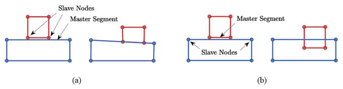
Example: The figures above show simple examples of master-slave contact between two elements (both are linear 4 noded small strain elements with a hypoelastic material model).   The base of the larger, bottom element is prevented from displacing vertically, and the leftmost node on the base is fixed. A prescribed vertical displacement is applied to the two nodes at the top of the upper, smaller element, and a horizontal displacement is imposed on its leftmost upper node.   Fig. (a) shows that when upper surface of the larger element is selected as master surface, the contact element correctly enforces the zero penetration boundary condition at the contact between the two (deformed) elements, while allowing the two to slide parallel to the contact.  Fig. (b) shows that switching master and slave element can sometimes affect the behavior of contact elements.   When the base of the smaller element is selected as the master surface, as in Fig (b), the slave nodes on the larger base element do not contact the master surface, and the overlap between the two elements is not detected.    This is a somewhat extreme example, but in general good mesh design will improve both the accuracy and convergence of a finite element simulation of contact between two or more solids.

 

A code that runs the test in this example is provided in the file FEM_Contact.m (along with input file Contact_example.txt) on the github site at

https://github.com/albower/Applied_Mechanics_of_Solids/