9.3 Modeling failure by crack growth $–$ linear elastic fracture mechanics

 

Phenomenological damage models are useful in design applications, but they have many limitations, including

 

· They require extensive experimental testing to calibrate the model for each application;

 

· They provide no insight into the relationship between a materials microstructure and its strength.

 

A more sophisticated approach is to model the mechanisms of failure directly.  Crack propagation through the solid, either as a result of fatigue, or by brittle or ductile fracture, is by far the most common cause of failure.  Consequently much effort has been devoted to developing techniques to predict the behavior of cracks in solids.  Below, we outline some of the most important results.

 

 

 

9.3.1 Crack tip fields in an isotropic, linear elastic solid.

 

Many of the techniques of fracture mechanics rely on the assumption that, if one gets sufficiently close to the tip of the crack, the stress, displacement and strain fields always have the same distribution, regardless of the geometry of the solid and how it is loaded.  The fields near a crack tip are a fundamental result in fracture mechanics.

 

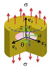
The figure shows (part of!) an infinitely large linear elastic solid, with Young’s modulus E and Poisson’s ratio $\nu$, which contains a crack.  The solid is loaded at infinity.  Note that

 

· Crack tip fields are most conveniently expressed in terms of cylindrical-polar coordinates $(r,\theta ,z)$ with origin at the crack tip;

 

· The displacement and stress near the crack tip can be characterized by three numbers $K_I,K_{II},K_{III}$, known as stress intensity factors. By definition

$K_I=\underset{r\to 0}{\lim }\sqrt{2\pi r}{\sigma }_{22}{K}_{II}=\underset{r\to 0}{\lim }\sqrt{2\pi r}{\sigma }_{12}{K}_{III}=\underset{r\to 0}{\lim }\sqrt{2\pi r}{\sigma }_{32}$

with the limit taken along $\theta =0$.

 

· The stress intensity factors depend on the detailed shape of the solid, and the way that it is loaded. To calculate stress intensity factors, you need to find the full stress field in the solid, and then compute the limiting values in the definition.  These calculations can be difficult $–$ you can try to find the solution in standard tables of stress intensity factors, or if this fails use a numerical method (such as FEM). A short table of stress intensity factors for various crack geometries can be found in Section 9.3.3, and FEM techniques are discussed in 9.3.4.

· Stress intensity factors have the bizarre units of $N{m}^{-3/2}$.

 

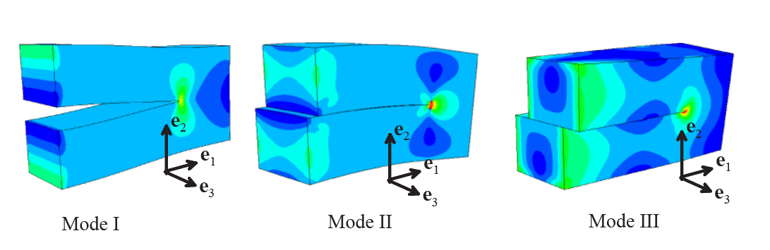
· The physical significance of the three stress intensity factors is illustrated below. The `Mode I’ stress intensity factor $K_I$ quantifies the crack opening displacements and stresses; the `Mode II’ stress intensity factor characterizes in-plane shear displacements and stress; and the `Mode III’ stress intensity factor quantifies out-of-plane shear displacement of the crack faces and anti-plane shear stresses at the crack tip.

 

 

 

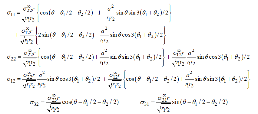
The stress field near the crack tip is

$\begin{array}{l}{\sigma }_{rr}={\displaystyle \frac{K_I}{\sqrt{2\pi r}}\left({\displaystyle \frac{5}{4}\cos {\displaystyle \frac{\theta }{2}-{\displaystyle \frac{1}{4}\cos {\displaystyle \frac{3\theta }{2}}}}}\right)+{\displaystyle \frac{K_{II}}{\sqrt{2\pi r}}\left(-{\displaystyle \frac{5}{4}\sin {\displaystyle \frac{\theta }{2}+{\displaystyle \frac{3}{4}\sin {\displaystyle \frac{3\theta }{2}}}}}\right)}}\\ {\sigma }_{\theta \theta }={\displaystyle \frac{K_I}{\sqrt{2\pi r}}\left({\displaystyle \frac{3}{4}\cos {\displaystyle \frac{\theta }{2}+{\displaystyle \frac{1}{4}\cos {\displaystyle \frac{3\theta }{2}}}}}\right)-{\displaystyle \frac{K_{II}}{\sqrt{2\pi r}}\left({\displaystyle \frac{3}{4}\sin {\displaystyle \frac{\theta }{2}+{\displaystyle \frac{3}{4}\sin {\displaystyle \frac{3\theta }{2}}}}}\right)}}\\ {\sigma }_{r\theta }={\displaystyle \frac{K_I}{\sqrt{2\pi r}}\left({\displaystyle \frac{1}{4}\sin {\displaystyle \frac{\theta }{2}+{\displaystyle \frac{1}{4}\sin {\displaystyle \frac{3\theta }{2}}}}}\right)+{\displaystyle \frac{K_{II}}{\sqrt{2\pi r}}\left({\displaystyle \frac{1}{4}\cos {\displaystyle \frac{\theta }{2}+{\displaystyle \frac{3}{4}\cos {\displaystyle \frac{3\theta }{2}}}}}\right)}}\end{array}$

Equivalent expressions in rectangular coordinates are

$\begin{array}{l}{\sigma }_{11}={\displaystyle \frac{K_I}{\sqrt{2\pi r}}\cos {\displaystyle \frac{\theta }{2}\left(1-\sin {\displaystyle \frac{\theta }{2}\sin {\displaystyle \frac{3\theta }{2}}}\right)-{\displaystyle \frac{K_{II}}{\sqrt{2\pi r}}\sin {\displaystyle \frac{\theta }{2}\left(2+\cos {\displaystyle \frac{\theta }{2}\cos {\displaystyle \frac{3\theta }{2}}}\right)}}}}\\ {\sigma }_{22}={\displaystyle \frac{K_I}{\sqrt{2\pi r}}\cos {\displaystyle \frac{\theta }{2}\left(1+\sin {\displaystyle \frac{\theta }{2}\sin {\displaystyle \frac{3\theta }{2}}}\right)+{\displaystyle \frac{K_{II}}{\sqrt{2\pi r}}\cos {\displaystyle \frac{\theta }{2}\sin {\displaystyle \frac{\theta }{2}\cos {\displaystyle \frac{3\theta }{2}}}}}}}\\ {\sigma }_{12}={\displaystyle \frac{K_I}{\sqrt{2\pi r}}\cos {\displaystyle \frac{\theta }{2}\sin {\displaystyle \frac{\theta }{2}\cos {\displaystyle \frac{3\theta }{2}+{\displaystyle \frac{K_{II}}{\sqrt{2\pi r}}\cos {\displaystyle \frac{\theta }{2}\left(1-\sin {\displaystyle \frac{\theta }{2}\sin {\displaystyle \frac{3\theta }{2}}}\right)}}}}}}\\ {\sigma }_{31}=-{\displaystyle \frac{K_{III}}{\sqrt{2\pi r}}\sin \theta /2{\sigma }_{32}={\displaystyle \frac{K_{III}}{\sqrt{2\pi r}}\cos \theta /2}}\end{array}$

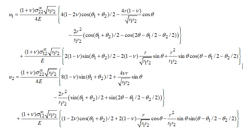
while the displacements can be calculated by integrating the strains, with the result

$\begin{array}{l}{u}_1={\displaystyle \frac{K_I}{\mu }\sqrt{{\displaystyle \frac{r}{2\pi }}}\left[1-2\nu +{\sin }^2{\displaystyle \frac{\theta }{2}}\right]\cos {\displaystyle \frac{\theta }{2}+{\displaystyle \frac{K_{II}}{\mu }\sqrt{{\displaystyle \frac{r}{2\pi }}}\left[2-2\nu +{\cos }^2{\displaystyle \frac{\theta }{2}}\right]\sin {\displaystyle \frac{\theta }{2}}}}}\\ u_2={\displaystyle \frac{K_I}{\mu }\sqrt{{\displaystyle \frac{r}{2\pi }}}\left[2-2\nu -{\cos }^2{\displaystyle \frac{\theta }{2}}\right]\sin {\displaystyle \frac{\theta }{2}+{\displaystyle \frac{K_{II}}{\mu }\sqrt{{\displaystyle \frac{r}{2\pi }}}\left[-1+2\nu +{\sin }^2{\displaystyle \frac{\theta }{2}}\right]\cos {\displaystyle \frac{\theta }{2}}}}}\\ u_3={\displaystyle \frac{K_{III}}{\mu }\sqrt{{\displaystyle \frac{2r}{\pi }}}\sin \theta /2}\end{array}$

Note that the formulas for in-plane displacement components $u_1,u_2$ are valid for plane strain deformation only.

 

 

 

9.3.2 The assumptions and application of phenomenological linear elastic fracture mechanics

 

The objective of linear elastic fracture mechanics is to predict the critical loads that will cause a crack in a solid to grow.  For applications involving fatigue or dynamic fracture, the rate and direction of crack growth are also of interest.

 

The phenomenological theory is based on the following qualitative argument.  Consider a crack in a reasonably brittle, isotropic solid.  If the solid were ideally elastic, we expect the asymptotic solution listed in the preceding section to become progressively more accurate as we approach the crack tip.  Away from the crack tip, the fields are influenced by the geometry of the solid and boundary conditions, and the asymptotic crack tip field is not accurate.  In practice, the asymptotic field will also not give an accurate representation of the stress fields very close to the crack tip. The crack may not be perfectly sharp at its tip, and if it were, no solid could withstand the infinite stress predicted by the asymptotic linear elastic solution.  We therefore anticipate that in practice the linear elastic solution will not be accurate very close to the crack tip itself, where material nonlinearity and other effects play an important role.  So the stress and strain distributions will have 3 general regions, as shown in the figure.

 

1. Close to the crack tip, there will be a process zone, where the material suffers irreversible damage. 

 

2. A bit further from the crack tip, there will be a region where the linear elastic asymptotic crack tip field might be expected to be accurate.  This is known as the `region of K dominance’

 

3. Far from the crack tip the stress field depends on the geometry of the solid and boundary conditions.

 

 

Material failure (crack growth or fatigue) is a consequence of the ugly stuff that goes on in the process zone.  Linear elastic fracture mechanics postulates that we don’t need to understand this ugly stuff in detail, since the fields in the process zone are likely to be controlled mainly by the fields in the region of K dominance.  The fields in this region depend only on the three stress intensity factors $K_I,K_{II},K_{III}$.  Therefore, the state in the process zone can be characterized by the three stress intensity factors.

 

If this is true, the conditions for crack growth, or the rate of crack growth, will be only a function of stress intensity factor and nothing else.  We can measure the critical value of $K_I,K_{II},K_{III}$ required to cause the crack to grow in a standard laboratory test, and use this as a measure of the resistance of the solid to crack propagation.  For fatigue tests, we can measure crack growth rate as a function of $K_I,K_{II},K_{III}$ or their history, and characterize the relationship using appropriate phenomenological laws.

 

Having characterized the material, we can then estimate the safety of a structure or component that containing a crack.  To do so, calculate the stress intensity factors for the crack in the structure, and then use our phenomenological fracture or fatigue laws to decide whether or not the crack will grow.

 

For example, the fracture criterion under mode I loading is written

$K_I\ge K_{IC}$

for crack growth, where $K_{IC}$ is the critical stress intensity factor for the onset of fracture.  The critical stress intensity factor is referred to as the Mode I fracture toughness of the solid.

 

Experimentally, it is found that this approach works quite well, provided that the assumptions inherent in linear elastic fracture mechanics are satisfied.

 

Careful tests and computer simulations have established the following conditions for the applicability of linear elastic fracture mechanics. A representative test specimen is sketched on the right. To measure an accurate value of toughness:

 

1. All characteristic specimen dimensions must exceed 25 times the expected plastic zone size at the crack tip;

 

2. For plane strain conditions at the crack tip the specimen thickness B must exceed at least the plastic zone size.

 

For a material with yield stress Y, loaded in Mode I with stress intensity factor $K_I$ the plastic zone size can be estimated as

$r_p\sim 2.5{\left({\displaystyle \frac{K_I}{Y}}\right)}^2$

 

 

Practical application of linear elastic fracture mechanics to in design

 

To apply LEFM in a design application, you need to be able to: 

 

1. Design a laboratory specimen that can induce a prescribed stress intensity factor at a crack tip

 

2. Measure the critical stress intensity factors that cause fracture in the laboratory specimen, or measure fatigue crack growth rates as a function of static or cyclic stress intensity

 

3. Estimate the anticipated size and location of cracks in your structure or component

 

4. Calculate the stress intensity factors for the cracks in your structure or component under anticipated loading conditions

 

5. Combine the results of steps 2 and 4 to predict the behavior of the cracks in the structure of interest, and make appropriate design recommendations.

 

 

These steps are outlined in more detail below.

 

 

9.3.3 Calculating stress intensity factors

 

Calculating stress intensity factors is a critical step in fracture mechanics.  Various techniques can be used to do this, including

 

1. Solve the full linear elastic boundary value problem for the specimen or component containing a crack, and deduce stress intensities from the asymptotic behavior of the stress field near the crack tips;

 

2. Attempt to deduce stress intensity factors directly using energy methods or path independent integrals, to be discussed in Section 9.4;

 

3. Look up the solution you need in tables;

 

4. Use a numerical method $–$ boundary integral equation methods are particularly effective for crack problems, but FEM can be used too.

 

 

 

Analytical solutions to some crack problems

 

Calculating stress intensity factors for a crack in a structure or component involves the solution of a standard linear elastic boundary value problem.  Once the stresses have been computed, the stress intensity factor is deduced from the definitions given in Section 9.3.1.  Exact solutions are known for a few simple geometries.  A couple of examples are listed below.

 

 

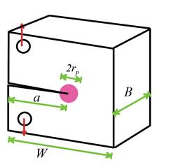
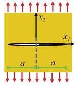
2D Slit crack in an infinite solid: The figure above shows a 2D crack with length 2a in an infinite solid, which is subjected to a uniform state of stress ${\sigma }_{22}^{\infty },{\sigma }_{12}^{\infty },{\sigma }_{32}^{\infty }$ at infinity.  The complex variable solution to this problem can be found in Section 5.3.  The solution is most conveniently expressed in terms of the polar coordinates $(r,\theta )$ centered at the origin, together with the auxiliary angles and distances $r_1,{\theta }_1$ and $r_2,{\theta }_2$ shown in the figure.  When evaluating the formulas, the angles ${\theta }_1$ and ${\theta }_2$ must lie in the ranges $-\pi \le {\theta }_1\le \pi 0\le {\theta }_2\le 2\pi$, respectively.  The complete displacement and stress fields in the solid are

 

 

 

The stress intensity factors are easily computed to be

$K_I={\sigma }_{22}^{\infty }\sqrt{\pi a}{K}_{II}={\sigma }_{12}^{\infty }\sqrt{\pi a}$       $K_{III}={\sigma }_{32}^{\infty }\sqrt{\pi a}$

 

 

Penny shaped crack in an infinite solid The figure above shows a circular crack with radius a in an infinite solid, subjected to uniaxial tension at infinity.  The displacement field, in cylindrical-polar coordinates, is

$u_r=-{\displaystyle \frac{\nu \sigma r}{E}+{\displaystyle \frac{(1+\nu )\sigma r}{\pi E}\left\{(1-2\nu )\left({\displaystyle \frac{a\sqrt{{\rho }_2^2-a^2}}{{\rho }_2^2}-{\sin }^{-1}{\displaystyle \frac{a}{{\rho }_2}}}\right)+{\displaystyle \frac{2a^2\left|z\right|\sqrt{a^2-{\rho }_1^2}}{{\rho }_2^2\left({\rho }_2^2-{\rho }_1^2\right)}}\right\}}}$

$u_z={\displaystyle \frac{\sigma z}{E}+{\displaystyle \frac{2(1+\nu )}{\pi E}\left\{2(1-\nu )\left({\displaystyle \frac{z}{\left|z\right|}\sqrt{a^2-{\rho }_1^2}-z{\sin }^{-1}{\displaystyle \frac{a}{{\rho }_2}}}\right)+z\left({\sin }^{-1}{\displaystyle \frac{a}{{\rho }_2}-{\displaystyle \frac{\sqrt{{\rho }_2^2-a^2}}{{\rho }_2^2-{\rho }_1^2}}}\right)\right\}}}$

$\begin{array}{l}{\rho }_1={\displaystyle \frac{1}{2}\left(\sqrt{{\left(a+r\right)}^2+z^2}-\sqrt{{\left(a-r\right)}^2+z^2}\right)}\\ {\rho }_2={\displaystyle \frac{1}{2}\left(\sqrt{{\left(a+r\right)}^2+z^2}+\sqrt{{\left(a-r\right)}^2+z^2}\right)}\end{array}$

These expressions are valid for z>0, the solution for z<0 can be found by symmetry.  The displacement of the upper crack face can be found by setting $r<a,z=0$ in these expressions, which gives

$u_z={\displaystyle \frac{4(1-{\nu }^2)\sigma }{\pi E}\sqrt{a^2-r^2}}$

The stress intensity factor can be found directly from the displacement of the crack faces.  The asymptotic formulas in 9.3.1 show that

$K_I=\underset{r\to a}{\lim }{\displaystyle \frac{E{u}_z(r)}{4(1-{\nu }^2)}\sqrt{{\displaystyle \frac{2\pi }{(a-r)}}}}$

which shows that $K_I=2\sigma \sqrt{a/\pi }$

 

It is not always necessary to solve the full linear elastic boundary value problem in order to compute stress intensity factors.  Energy methods, or the application of path independent integrals, can sometimes be used to obtain stress intensity factors directly.  These techniques will be discussed in more detail in Section 9.4.

 

Vast numbers of crack problems have been solved to catalog stress intensity factors in various geometries of interest.  Two excellent (but expensive) sources of such solutions are Tada (2000) and Murakami (1987).  A few important (and relatively simple) results are listed in the table below.

 

 

 

Calculating stress intensity factors for cracks in nonuniform stress fields

 

The solutions for cracks loaded by point forces acting on their faces are particularly useful, because they allow you to calculate stress intensity factors for a crack in an arbitrary stress field using a simple superposition argument.  The procedure works like this. 

 

1. We start by computing the stress field in a solid without a crack in it.  This solution satisfies all boundary conditions except that the crack faces are subject to tractions

 

2. We could correct solution by applying pressure (and shear) to the crack faces that are just sufficient to remove the unwanted tractions.

 

 

3. If we know the stress intensity factors induced by point forces acting on the crack faces, we can superpose an appropriate distribution of point forces on the crack faces calculate stress intensity factors induced by the corrective pressure distribution.

 

 

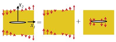
As an example, suppose that we want to calculate stress intensity factors for a crack in a linearly varying stress field (such as would be induced by bending a beam, for example), as illustrated above.

 

1. In the uncracked solid, the stress field is  ${\sigma }_{22}={\sigma }_0{x}_1/L$

 

2. The traction acting along the line of the crack is $p={\sigma }_0{x}_1/L$ The sign convention for p is that a positive p acts downwards on the upper crack face, and upwards on the lower crack face

 

 

3. To remove the traction from the crack faces, we must superpose an equal and opposite distribution of point forces on the crack faces.  The stress intensity factor induced at the left (L) and right (R) crack tips are

$K_I^R={\displaystyle \frac{1}{\sqrt{\pi a}}{\displaystyle \underset{-a}{\overset{a}{\int }}({\sigma }_0{x}_1/L)\sqrt{{\displaystyle \frac{a+x_1}{a-x_1}}}}d{x}_1{K}_I^L={\displaystyle \frac{1}{\sqrt{\pi a}}{\displaystyle \underset{-a}{\overset{a}{\int }}({\sigma }_0{x}_1/L)\sqrt{{\displaystyle \frac{a-x_1}{a+x_1}}}}d{x}_1}}$

Evaluating the integrals gives

$K_I^R={\displaystyle \frac{1}{2}({\sigma }_0/L)a\sqrt{\pi a}{K}_I^L=-{\displaystyle \frac{1}{2}({\sigma }_0/L)a\sqrt{\pi a}}}$

 

Actually, this solution is not quite right - note that the stress intensity factor at the left crack tip is predicted to be negative.  This cannot be correct $–$ from the asymptotic stress field we know that if the stress intensity factor is negative, the crack faces must overlap behind the crack tip (the displacement jump is negative). 

 

 

With a bit of cunning, we can fix this problem.  The cause of the error in the quick estimate is that we removed tractions from the entire crack $–$ this was a mistake; we should only have removed tractions from parts of the crack faces that open up.   So let’s suppose that the crack closes at $x_1=-b$, and put the left hand crack tip there (see the figure on the right). The stress intensity factors are then

$\begin{array}{l}{K}_I^R={\displaystyle \frac{1}{\sqrt{\pi (a+b)/2}}{\displaystyle \underset{-b}{\overset{a}{\int }}({\sigma }_0{x}_1/L)\sqrt{{\displaystyle \frac{b+x_1}{a-x_1}}}}d{x}_1}\\ K_I^L={\displaystyle \frac{1}{\sqrt{\pi (a+b)/2}}{\displaystyle \underset{-b}{\overset{a}{\int }}({\sigma }_0{x}_1/L)\sqrt{{\displaystyle \frac{a-x_1}{b+x_1}}}}d{x}_1}\end{array}$

This gives

$K_I^L={\displaystyle \frac{({\sigma }_0/L)\sqrt{2\pi }}{8\sqrt{(a+b)}}\left(a^2-2ab-3b^2\right)}$

for the stress intensity factor at the left hand crack tip.  The stress must be bounded at $x_1=-b$ where the crack faces touch, so that $K_I^L=0$.  This gives $b=a/3$.  The stress intensity factor at the right hand crack tip then follows as

$$ $K_I^R={\displaystyle \frac{2({\sigma }_0/L)a\sqrt{6\pi a}}{9}}$

This is not very different to our earlier estimate.  This illustrates a general feature of the field of fracture mechanics.  There are many opportunities to do clever things, but often the results of all the cleverness are irrelevant.

 

 

 

9.3.4 Calculating stress intensity factors using finite element analysis

 

For solids with a complicated geometry, finite element methods (or boundary element methods) are the only way to calculate stress intensity factors.  It is conceptually very straightforward to calculate stress intensities using finite elements $–$ you just need to solve a routine linear elastic boundary value problem to determine the stress field in the solid, and then deduce the stress intensity factors by taking the limits given in Section 9.3.1.

 

Unfortunately, this is easier said than done.  The problem is that the stress and strain fields at a crack tip are infinite, and so standard finite element methods have problems calculating the stresses accurately.  Two special procedures have been developed to help deal with this:

 

1. Special crack tip elements are available to approximate the singular strains at a crack tip;

 

2. Special techniques are available to calculate stress intensity factors from stresses far from the crack tip (where they should be accurate) instead of using the formal definition.

 

These methods can both give very accurate values for stress intensity factors $–$ and can be used together to obtain the best results.

 

 

Crack tip elements

 

A very simple procedure can be used to approximate the strain singularity at a crack tip.

 

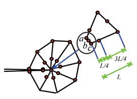
1. The solid near the crack tip must be meshed with quadratic elements (8 noded quadrilaterals or 6 noded triangles in 2D, or 20 noded bricks/10 noded tetrahedral in 3D). 

 

2. The elements connected to the crack tip must be quadrilateral or brick elements

 

3. One side of each element connected to the crack tip is collapsed to make the three nodes on the side coincident, as shown in the figure.

 

4. The mid-side nodes on the elements connected to the crack tip are shifted to $\mathrm{¼}$ point positions, as shown in the figure.

 

5. If the coincident nodes a,b,c on each crack-tip element are constrained to move together, this procedure generates a ${\left(r\right)}^{-1/2}$ singularity in strain at the crack tip (good for linear elastic problems).  If the nodes are permitted to move independently, a $r^{-1}$ singularity in strain is produced (good for problems involving crack tip plasticity)

 

 

 

Calculating stress intensity factors using path independent integrals

 

Energy methods in fracture mechanics are discussed in detail in Section 9.4.  Two crucial results emerge from this analysis

 

1. The ‘energy release rate’ for a mode I crack in a linear elastic solid with Young’s modulus E and Poisson’s ratio $\nu$ is related to the mode I stress intensity factor by

$G={\displaystyle \frac{1-{\nu }^2}{E}{K}_I^2}$

 

2. The energy release rate for a crack can be calculated by evaluating the following line integral for any contour that starts on one crack face and ends on the other

$G={\displaystyle \underset{\Gamma }{\int }(W{\delta }_{j1}-{\sigma }_{ij}{\displaystyle \frac{\partial u_i}{\partial x_1})m_{j}ds}}$

where $W={\sigma }_{ij}{\epsilon }_{ij}/2$ is the strain energy density, ${\sigma }_{ij}$ is the stress field, $u_i$ is the displacement field, $m_i$ is a unit vector normal to $\Gamma$, and the $e_1$ basis vector is parallel to the direction of crack propagation as shown in the figure.

 

These results are ideally suited for FEM calculations.  The path independent integral can be calculated for a contour far from the crack tip, where the stresses are accurate, and then the relationship between G and $K_I$ can be used to deduce the stress intensity factors.  Analogous, but rather more complex, procedures exist to extract all three components of stress intensity factor, as well as to compute stress intensity factors for 3D cracks, where the stress intensity factor is a function of position on the crack front.   There is also a technique that transforms the line integral into an equivalent area integral, which can also be evaluated easily in a finite element code.

 

 

 

9.3.5 Measuring fracture toughness

 

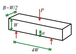
For structural applications, standard testing techniques are available to measure material properties for fracture applications.  Two standard test specimen geometries are shown below. Stress intensity factors for these specimens have been carefully computed as a function of crack length and the results fit by curves, as outlined below

 

Compact tension specimen (shown above)

 

 

$\begin{array}{l}{K}_I={\displaystyle \frac{P}{B}\sqrt{{\displaystyle \frac{\pi }{W}}}\left\{16.7{\left({\displaystyle \frac{a}{W}}\right)}^{1/2}-104.7{\left({\displaystyle \frac{a}{W}}\right)}^{3/2}+369.9{\left({\displaystyle \frac{a}{W}}\right)}^{5/2}\right.}\\ \left.-573.8{\left({\displaystyle \frac{a}{W}}\right)}^{7/2}+360.5{\left({\displaystyle \frac{a}{W}}\right)}^{9/2}\right\}\end{array}$

 

Three point bend specimen

 

 

$\begin{array}{l}{K}_I={\displaystyle \frac{4P}{B}\sqrt{{\displaystyle \frac{\pi }{W}}}\left\{1.6{\left({\displaystyle \frac{a}{W}}\right)}^{1/2}-2.6{\left({\displaystyle \frac{a}{W}}\right)}^{3/2}+12.3{\left({\displaystyle \frac{a}{W}}\right)}^{5/2}\right.}\\ \left.-21.2{\left({\displaystyle \frac{a}{W}}\right)}^{7/2}+21.8{\left({\displaystyle \frac{a}{W}}\right)}^{9/2}\right\}\end{array}$

 

Various other test specimens exist.

 

Conducting a fracture test or fatigue test is (at least conceptually) straightforward $–$ you make a specimen (for fracture tests a sharp crack is usually created by initiating a fatigue crack at the tip of a notch); and load it in a tensile testing machine.

 

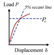
 In principle, the fracture toughness can be determined by measuring the critical load when the crack starts to grow.  In practice it can be difficult to detect the onset of crack growth.  For this reason, the usual approach is to monitor the crack opening displacement $\delta$ during the test, then plot load as a function of crack opening displacement.  A typical result is illustrated in the figure.

 

The load-CTOD curve ceases to be linear when the crack begins to grow.  This point is hard to identify, so instead the convention is to draw a line with slope 5% lower than the initial $P-\delta$ curve (the 5% secant line) and use the point where this line intersects the $P-\delta$ as the fracture load. The plane strain fracture toughness of the material, $K_{IC}$, is deduced from the fracture load, using the calibration for the specimen.

 

After measurement, one must check that $K_{IC}$ is within the limits required for K dominance in the specimen, following the rules in the preceding section.

 

 

 

9.3.6 Typical values for fracture toughness

 

A short table of approximate toughness values is given in Table 9.3 (see Jones and Ashby, 2019 for a more extensive list).  The values are highly dependent on material composition and microstructure, however, so if you need accurate data you will need to measure the toughness of your materials yourself.

 

 

 

 

9.3.7 Stable Tearing $–$ Kr curves and Crack Stability

 

In ideally brittle materials, fracture is a catastrophic event.  Once the load reaches the level required to trigger crack growth, the crack continues to propagate dynamically through the specimen.  In more ductile materials, a period of stable crack growth under steadily increasing load may occur prior to complete failure.  This behavior is particularly common in tearing of thin sheets of metals, but stable crack growth is observed in most materials $–$ even polycrystalline ceramics.

 

Stable crack growth in metals usually occurs because a zone of plastically deformed material is left in the wake of the crack, as shown in the figure. This deformed material tends to reduce the stresses at the crack tip.  In brittle polycrystalline ceramics, or in fiber reinforced brittle composites, the stable crack growth is caused by the formation of a `bridging zone’ behind the crack tip.  Some fibers, or grains, remain intact in the crack wake, and tend to hold the crack faces shut, increasing the apparent strength of the solid.

 

In some materials, the increase in load during stable crack growth is so significant that it’s worth accounting for the effect in design calculations.  The protective effect of the process zone in the crack wake is modeled by making the toughness of the material a function of the increase in crack length.  The apparent toughness is measured in the same way as $K_{IC}$ - a pre-cracked specimen is subjected to progressively increasing load, and the crack length is monitored either optically or using compliance methods (more on this later).  A value of $K_I$ can be computed for the specimen using the calibrations $–$ during crack growth it is assumed that $K_I$ is equal to the fracture toughness of the material.

 

The results are plotted in a `resistance curve’ or `R curve’ for the material, as shown below. The fracture toughness $K_{IC}$ is the critical stress intensity factor required to initiate crack growth.  The variation of toughness with crack growth is denoted $K_r(\Delta a)$.

 

 

The resistance curve is then used to predict the conditions necessary for unstable crack growth through the material.  To see how this is done

 

1. Consider a large sample of material containing a slit crack of length 2a, subjected to stress $\sigma$, as shown on the right. The stress intensity factor for this crack (from the table in sect 9.3.3) is $K_I=\sigma \sqrt{\pi a}$.

 

2. Crack growth begins when $\sigma \sqrt{\pi a}=K_{IC}$.   Thereafter, there will be a period of stable crack growth, during which the applied stress increases.  During the period of stable growth the stress intensity factor must equal the apparent toughness

$\sigma \sqrt{\pi (a+\Delta a)}=K_r\left(\Delta a\right)\Rightarrow \sigma ={\displaystyle \frac{K_r\left(\Delta a\right)}{\sqrt{\pi (a+\Delta a)}}}$

3. The stress will continue to increase as long as $K_r(\Delta a)$ increases more rapidly than $\sqrt{\pi (a+\Delta a)}$ with $\Delta a$.  Catastrophic failure (unstable crack growth) will occur when continued crack growth is possible at constant or decreasing load.  The crack length at the point of unstable crack growth follows from the condition that

${\displaystyle \frac{d\sigma }{d\Delta a}=0\Rightarrow a+\Delta a={\displaystyle \frac{K_r}{2(d{K}_r/d\Delta a)}{\displaystyle \frac{d{K}_r}{d\Delta a}}}}$

 

4. Substituting the crack length back into the fracture criterion $\sigma \sqrt{\pi (a+\Delta a)}=K_r\left(\Delta a\right)$ gives the critical stress at unstable fracture as

$\sigma =\sqrt{{\displaystyle \frac{2}{\pi }{K}_r{\displaystyle \frac{d{K}_r}{d\Delta a}}}}$

 

 

 

9.3.8 Mixed Mode fracture criteria

 

Fracture toughness is almost always measured under mode I loading (except when measuring fracture toughness of a bi-material interface).  If a crack is subjected to combined mode I and mode II loading, a mixed mode fracture criterion is required.  There are several ways to construct mixed mode fracture criteria $–$ the issue has been the subject of some quite heated arguments.  The criterion of maximum hoop stress is one example.  Recall that the crack tip hoop and shear stresses are

$\begin{array}{l}{\sigma }_{\theta \theta }={\displaystyle \frac{K_I}{\sqrt{2\pi r}}\left({\displaystyle \frac{3}{4}\cos {\displaystyle \frac{\theta }{2}+{\displaystyle \frac{1}{4}\cos {\displaystyle \frac{3\theta }{2}}}}}\right)-{\displaystyle \frac{K_{II}}{\sqrt{2\pi r}}\left({\displaystyle \frac{3}{4}\sin {\displaystyle \frac{\theta }{2}+{\displaystyle \frac{3}{4}\sin {\displaystyle \frac{3\theta }{2}}}}}\right)}}\\ {\sigma }_{r\theta }={\displaystyle \frac{K_I}{\sqrt{2\pi r}}\left({\displaystyle \frac{1}{4}\sin {\displaystyle \frac{\theta }{2}+{\displaystyle \frac{1}{4}\sin {\displaystyle \frac{3\theta }{2}}}}}\right)+{\displaystyle \frac{K_{II}}{\sqrt{2\pi r}}\left({\displaystyle \frac{1}{4}\cos {\displaystyle \frac{\theta }{2}+{\displaystyle \frac{3}{4}\cos {\displaystyle \frac{3\theta }{2}}}}}\right)}}\end{array}$

The maximum hoop stress criterion postulates that a crack under mixed mode loading starts to propagate when the greatest value of hoop stress ${\sigma }_{\theta \theta }$ reaches a critical magnitude, at which point the crack will branch at the angle for which ${\sigma }_{\theta \theta }$ is greatest (or equivalently the angle for which ${\sigma }_{r\theta }=0$ ).  The critical angle is plotted as a function of $K_{II}/K_I$ below.  The asymptote for $K_{II}/K_I\to \infty$ is -70.7 degrees.  The resulting failure locus (the critical combination of $K_I/K_{IC}$ and $K_{II}/K_{IC}$ that leads to failure) is also shown.

     

 

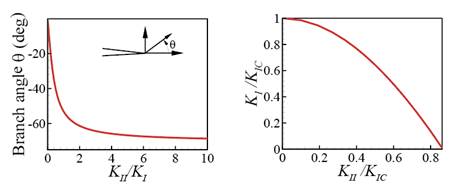
All available criteria predict that, after branching, a crack will follow a path such that the local mode II stress intensity factor is zero.

 

 

 

9.3.9 Static fatigue crack growth

 

For a fatigue test, the crack length is measured (optically, or using compliance techniques) as a function of time or number of load cycles. Fatigue laws are deduced by plotting crack growth rate as a function of applied stress intensity factor.

 

Typical static fatigue data (e.g. for corrosion crack growth, or creep crack growth) behavior is shown below

 

 

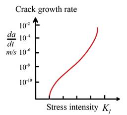
Most materials have a static fatigue threshold $–$ a value of $K_I$ below which crack growth is undetectable.  Then there is a range where crack growth rate shows a power-law dependence on stress intensity factor of the form

${\displaystyle \frac{da}{dt}=C{K}_I^m}$

where m is typically of order 5-10.  Finally, for values of $K_I$ approaching the fracture toughness, the crack growth rate increases drastically with $K_I$.

 

This crack growth law can be used to derive the phenomenological static fatigue criterion outlined in Section 8.2.3.    Assume that at time t=0 the material contains a crack of initial length $2a=2a_0$, and is subjected to a uniaxial stress $\sigma$, as on the right.   

 

The stress will cause the crack to increase in length, until it becomes long enough to trigger brittle fracture.  The table in Sect 9.3.9 below shows that a crack of length 2a subjected to stress $\sigma$ the stress has a crack tip stress intensity factor $K_I=\sigma \sqrt{\pi a}$.   Substituting into the static fatigue crack growth law and integrating gives the following expression for crack length as a function of time

${\displaystyle \frac{2}{m-2}\left({\displaystyle \frac{1}{a_0^{m/2-1}}-{\displaystyle \frac{1}{a^{m/2-1}}}}\right)=C{\pi }^{m/2}{\displaystyle \int {\sigma }^{m}dt}}$

where 2 $a_0$ is the crack length at time t=0.   The solid will fracture when the crack tip stress intensity factor reaches the fracture toughness $K_{IC}$, so that the tensile strength at time t=0   and at time t  must satisfy

${\sigma }_{TS0}\sqrt{\pi a_0}=K_{IC}{\sigma }_{TS}\sqrt{\pi a}=K_{IC}$

Eliminating the crack length and simplifying gives

${\sigma }_{TS}={\sigma }_{TS0}{\left(1-{\displaystyle \frac{(m-2)\pi C{K}_{IC}^{m-2}}{2{\sigma }_{TS0}^{m-2}}{\displaystyle \int {\sigma }^{m}dt}}\right)}^{1/(m-2)}$

Assuming that the operating stress is well below the fracture stress, we can approximate this by

${\sigma }_{TS}={\sigma }_{TS0}\left(1-\alpha {\displaystyle \int {\left(\sigma /{\sigma }_{TS0}\right)}^{m}dt}\right)$

which is the stress based static fatigue law of Sect 9.2.3.

 

 

 

 

9.3.10 Cyclic fatigue crack growth

 

Under cyclic loading, the crack is subjected to a cycle of mode I and mode II stress intensity factor. Most fatigue tests are performed under a steady cycle of pure mode I loading, as sketched below.

 

 

The results are usually displayed by plotting the crack growth per cycle $da/dN$ as a function of the stress intensity factor range

$\Delta K_I=\left\{\begin{array}{c}{K}_{\max }-K_{\min }{K}_{\min }\ge 0\\ K_{\max }{K}_{\min }<0\end{array}\right.$

 

A typical result shows three regions, as shown on the right. There is a fatigue threshold $\Delta K_{th}$ below which crack growth is undetectable.  For modest loads, the crack growth rate obeys Paris law

${\displaystyle \frac{da}{dN}=C{\left(\Delta K_I\right)}^n}$

where the index n is between 2 and 4.  As the maximum stress intensity factor approaches the fracture toughness of the material, the crack growth rate accelerates dramatically.

 

In the Paris law regime, the crack growth rate is only weakly sensitive to the mean value of stress intensity factor $K_m$.  In the other two regimes,  $K_m$ has a noticeable effect - the fatigue threshold is reduced as $K_m$ increases, and the crack growth rate in regime III increases with $K_m$. 

 

 

 

9.3.11 Finding cracks in structures

 

Determining the length of pre-existing cracks in a component is often the most difficult part of applying fracture mechanics in practice.  For most practical applications you simply don’t know if your component will have a crack in it, and it will be expensive if you need to find out.  Your options are:

 

1. Take a wild guess, based on microscopic examinations of representative samples of material.  Alternatively, you can specify the biggest flaw you are prepared to tolerate and insist that your material suppliers manufacture appropriately defect free materials.

 

2. Conduct a proof test (popular e.g. with pressure vessel applications) wherein the structure or component is subjected to a load greatly exceeding the anticipated service load under controlled conditions.  If the fracture toughness of the material is known, you can then deduce the largest crack size that could be present in the structure without causing failure during proof testing.

 

3. Use some kind of non-destructive test technique to attempt to detect cracks in your structure.  Examples of such techniques are ultrasound, where you look for echoes off crack surfaces; x-ray techniques; and inspection with optical microscopy.  If you detect a crack, most of these techniques will allow you to estimate the crack length.  If not, you have to assume for design purposes that your structure is crammed full of cracks that are just too short to be detected.