8.7 Structural
Elements: Two force members, Beams and Plates
It would take many millions of
three-dimensional continuum elements to mesh a structure such as a bridge or
building, even though the stress and strain fields within individual structural
members have a simple form. So, to make
computations easier and faster, special ‘structural elements’ are nearly always
used to model a complete structure of this kind. These elements all approximate the internal
stress and strain fields in the member in some appropriate way. In this section, we discuss a few commonly
used structural elements to illustrate their features.
8.7.1 Truss Elements.
 A truss consists of a set of bars
with a uniform cross-section, which are connected by pin joints. The structure may be loaded by applying
forces to some of the joints, while other joints may be fixed or subjected to a
known displacement. If the truss is in
static equilibrium, its members are all in a state of uniaxial tension or
compression. Each member can be regarded
as a single finite element (a ‘truss’ element), and the joints can be regarded
as the nodes connecting the elements.
The joint displacements are the unknown degrees of freedom.
A truss consists of a set of bars
with a uniform cross-section, which are connected by pin joints. The structure may be loaded by applying
forces to some of the joints, while other joints may be fixed or subjected to a
known displacement. If the truss is in
static equilibrium, its members are all in a state of uniaxial tension or
compression. Each member can be regarded
as a single finite element (a ‘truss’ element), and the joints can be regarded
as the nodes connecting the elements.
The joint displacements are the unknown degrees of freedom.
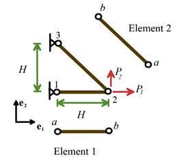
The figure shows a simple example of
a truss. The geometry of the structure is characterized by
1. The initial and final positions , of the N joints;
2. The joint displacements ;
3. The initial and deformed
cross-sectional area of the m
members;
4. The initial and final length of the members;
5. The axial and transverse stretch in
each member (with joints b and a at its two ends)
6. The axial component of infinitesimal
strain in each member
7. The axial component of stretch rate
in the member with joints a and b at its ends is given by
A set of external point forces act at the joints. The internal forces can be characterized by
the axial component of Cauchy stress in the members.
As usual, the finite element method
solves the static equilibrium equation by re-writing it as the equivalent
principle of virtual work. For this
purpose, we introduce a kinematically admissible virtual velocity for each joint (any displacement component
that is prescribed for a joint must have a zero virtual velocity). The virtual velocity has a corresponding
virtual stretch rate
The principal of virtual work is then
where the sums are taken over the members and loaded joints,
respectively.
Elastic structures with small displacements: Most practical structures are subjected to modest loads, so
their deformations are small and the members remain elastic. Under these conditions the strain in the
members can be approximated by the axial component of the infinitesimal strain , while the Cauchy stress is given by
, where E is the Young’s modulus of the member. In addition, changes in the the
cross-sectional area and length of the members can be neglected. The infinitesimal strain in the kth member can then be calculated from
the displacements of joints a and b at its two ends using the matrix
expression
Here, the vectors are 6 dimensional
(for a 3D structure), with the bold symbols representing either three position
vector components or three displacement components. You can multiply out the vector product to
see that this form is equivalent to the dot product in item (6) of the
preceding sub-section. The rate of
change of infinitesimal strain can replace the virtual stretch rate. Consequently, the principle of virtual work
can be written as
The virtual work equation must be
satisfied for all admissible joint velocities.
By choosing a set of virtual displacements in which only one
displacement component at one joint is nonzero in turn for all the joints yields
a system of linear equations
where the symbol denotes an ‘outer’ or dyadic product of the
two vectors, P represents a column
vector containing all the external forces, and the sum in the expression for
the stiffness represents the assembly of element stiffness matrices into a
global stiffness. After modifying the equations to account for any prescribed
displacements, they may be solved to determine the unknown joint displacements.
We can illustrate the procedure in
more detail using the simple 3-noded planar truss shown in the figure. The joints have coordinates
The two element stiffnesses are therefore
The element stiffnesses may be
combined into a 6x6 global stiffness to yield the (singular) equation system
Finally, the equation system must be
modified to ensure that the displacements at joints 1 and 3 are zero. Usually this is done so that the global
stiffness remains symmetric, in which case the final system of equations is
The system can be solved for the
unknown displacement at node 2 with the result
Trusses made from nonlinear elastic materials that experience large
displacements: More
generally, the members of the truss may be made from a rubbery material that
can be stretched significantly. It is
more difficult to calculate the deformation and internal forces in this kind of
structure, because the stress-strain relation and the equilibrium equation are
nonlinear.
As an example, consider a truss that
has its members made from an incompressible nonlinear elastic material with
uniaxial Cauchy stress-v-stretch relation Some specific stress-stretch relations for
rubber elasticity models are listed in Section 3.5.5: for example, the
‘neo-hookean’ material has a Cauchy stress
where is the shear modulus.
In a nonlinear structure, it is usually
helpful to calculate the joint displacements as the load is applied in a series
of increments. So, suppose that the
joint positions at a time instant t are known, and we wish to determine the new displacements at time .
The virtual work equation at is
where we have noted that ( is the stretch of the kth member), and that because the material is incompressible. The virtual equation must be satisfied for
all admissible virtual velocities, which yields a set of nonlinear equations
that must be solved numerically.
Nonlinear equilibrium equations in
finite element analysis are usually solved using Newton-Raphson iteration. For a truss, this means that we repeatedly
correct a current approximation for the joint displacements by an amount until the equilibrium equation is
satisfied. Ideally the correction
should satisfy , but of course it is not possible to
solve this equation, so instead we take a Taylor expansion and rearrange
This is now a set of linear equations
which, together with equations for joints with prescribed displacements, can be
solved for .
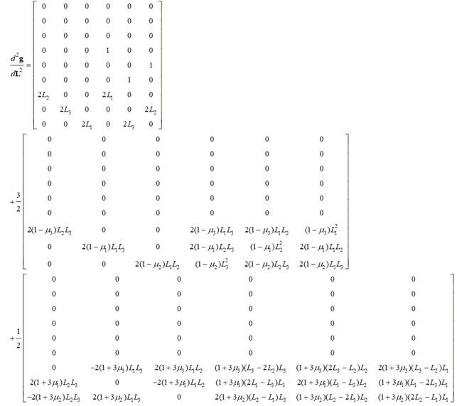
The stiffness matrix (prior to applying constraints) is
where I represents
a (3x3) identity matrix (for a 3D structure), and the summation represents the
assembly of the stiffness matrix for the k
th element (which has nodes (a,b) at
its two ends) into a global stiffness.
The Newton-Raphson equation solver
usually works well, but if the joint deflections are so large that the
structure ‘snaps through’ an unstable equilibrium configuration, it may fail to
converge. In this case a simple
iterative relaxation solver may work better.
This approach involves the following steps. Start with an initial guess for the joint
coordinates w (which is usually the
positions at the end of the preceding load-step). Then:
1. Update the coordinates of any joints
with prescribed displacements to their deformed positions;
2. Compute the force vector R;
3. Set rows of R corresponding to degrees of freedom with known displacements to
zero
4. Check for convergence (where TOL
is an appropriate small tolerance).
If the solution has converged update the joint coordinates to y=w and proceed to the next load-step.
5. If the solution has not yet
converged, updated the approximate joint positions to , where is a numerical relaxation factor (for the
neo-hookean material , where the max is taken over all
members) and proceed to step 2.
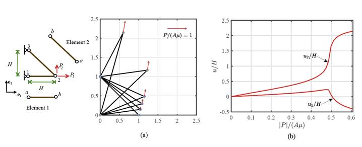
As an example, the figure above
illustrates the predicted deformation of a 3 noded truss structure (with
members made from a hyperelastic material with modulus ) subjected to horizontal and vertical forces
with ratio . Fig.
(a) shows the shape of the deformed structure for various magnitudes of the
applied force; while the graph (b) shows the displacement of the loaded joint
as a function of the magnitude of the force.
Trusses made from elastic-plastic materials that experience large
displacements: Finally,
we show how to analyze a truss that has its members made from a metallic
material, which displays elastic behavior at low stresses, and experiences
permanent plastic deformation if the stresses exceed yield.
Specifically, consider a truss with
members made from an elastic rate independent plastic material that
displays power law hardening. For this
type of material, the stretch in the members can be separated into a
reversible elastic part , and a permanent plastic part , so that .
The yield stress of the members is related to the accumulated plastic
strain by
where is the initial yield stress, m<1 is the strain hardening exponent,
and the accumulated plastic strain is related to the plastic stretch by
The uniaxial Cauchy (true) stress in
the members is related to the elastic part of the stretch by
where E is the Young’s modulus.
The plastic stretch rate is zero if the stress is below the yield
stress, or if the stress magnitude is decreasing. Otherwise, the plastic stretch rate is given
by
Changes in volume of the members can be neglected.
The virtual work equation and the
Newton-Raphson iterations for an elastic-plastic truss have the same form as
those listed for a hyperelastic truss in the preceding section. Only the expressions for the stress and its
derivative with respect to stretch need to be changed.
The stress-strain relation for a
plastically deforming material depends on the history of loading, so the finite
element solution must calculate the gradual change in shape of the structure as
the load is applied in a series of increments.
Suppose that at the start of the nth
time increment the plastic stretch and the total accumulated plastic strain
have values .
Given the total stretch at the end of the time step we must now
calculate at the end of the time-step. This can be accomplished using the following
(implicit) stress update:
1.
Calculate
the stress that would occur if the bar remains elastic, which is given by
.
2.
Check
whether the stress is below the yield stress: .
If this condition is satisfied, the bar remains elastic and the stress
is given by the formula in step 1. The
tangent is .
3. If the estimate for stress in step 1
exceeds the yield stress, the plastic stretch and the accumulated plastic
strain follow from the condition that the stress must equal the yield
stress. This requires
These two equations can be combined
to eliminate and then solved for using Newton-Raphson iteration (or any
convenient numerical method).
4.
The
stress follows as
5. Finally, a straightforward but
tedious calculation shows that the derivative of Cauchy stress with respect to
stretch is
A truss with elastic-plastic members
may experience a sudden loss of stability (particularly if the truss is
statically determinate). Because of the
instability, the Newton-Raphson solution to the virtual work equation may fail
to converge. The relaxation method
described in the preceding section can sometimes produce a better result.
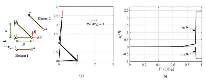
As an example, the figure illustrates
the predicted deformation of a 3 noded truss structure (with members made from
an elastic-plastic material with yield stress , Young’s modulus and hardening exponent ) subjected to horizontal and vertical forces
with ratio .
Fig. (a) shows the shape of the deformed structure for various
magnitudes of the applied force; while graph (b) shows the displacement of the
loaded joint as a function of the magnitude of the force.
8.7.2 Beam Elements.
A beam is a slender member, with uniform
(or slowly varying) cross-section, and length much greater than any
cross-sectional dimension. It may be
subjected to forces and moments at its ends, or transverse forces along its
length. These cause the beam to bend,
twist and stretch. But because it has a
slender cross-section, the stress and strain fields in a beam have a simple
form. There are two approaches to
analyzing deformation in an assembly of beams using the finite element method. The first is to set up and solve a finite
element approximation to the classical differential equations governing
deformation of a beam. These equations
were derived by approximating the strain field inside the beam in some
appropriate way, so these approximations are built into the finite element solution
from the beginning. This idea has two
limitations: (i) it works only if the beam remains elastic; and (ii) the most
common version of classical beam theory (Euler-Bernoulli theory) assumes that
planes transverse to the axis of the undeformed beam remain transverse to the
deformed beam axis. This is accurate
for beams with length exceeding about 10 times the beam thickness or width, but
not for shorter beams for short beams, ‘shear flexible’ (Timoshenko)
beam theory gives better results. It is
also possible to get around these limitations by meshing a beam with standard
3D (or 2D) isoparametric elements, but the mesh would need to include at least
5-10 elements through the thickness of the beam, and since the elements would
need to remain roughly cubic or square to avoid locking, a huge number of
elements would needed even to analyze a single beam. To avoid this, a better approach is to modify
isoparametric elements so that they produce the correct strain field in a
slender beam. These are called
‘continuum beam’ elements. Continuum beam theory in 3D is too complicated
to discuss here, but we will show how to implement finite element versions of
both Euler-Bernoulli and Timoshenko beam theory.
 Summary of beam theory: Beam theory is discussed in (tedious) detail in Chapter 10,
but to understand how to solve the equations using the finite element method,
only a short summary is needed.
Summary of beam theory: Beam theory is discussed in (tedious) detail in Chapter 10,
but to understand how to solve the equations using the finite element method,
only a short summary is needed.
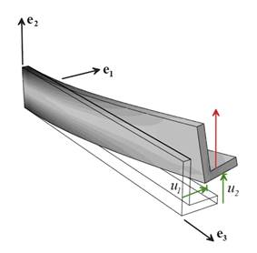
The figure shows a beam. We will assume that the beam is straight,
with a uniform cross-section, and is made from an isotropic elastic material
with Young’s modulus E and shear
modulus .
It experiences only small deformations.
It is often assumed that the beam does not
stretch or twist, but in the version described here we will account (approximately)
for both, but we will assume that sections of the beam that are transverse to
its axis remain plane. In practice,
twisting the rod will cause its cross-section to warp. The procedure necessary to correct for this
effect in an elastic beam is discussed in more detail in Chapter 10.
The geometry of the beam is usually
described using a basis shown in the figure, with is parallel to the beam’s axis, and orientated in some convenient direction with
respect to its cross section. We then
define the following geometrical quantities:
1. The cross-sectional area
2. The position of the neutral line in
the cross section (this is a fiber in the beam that does not stretch as the
beam bends)
3. The components of the area moment of
inertia tensor for the cross-section
The effects of warping can be included by replacing by a modified polar moment of area. The procedure is discussed in detail in
Chapter 10.
The deformed shape of a straight beam
is described by specifying the displacement of each point on the neutral line of the
cross-section, as a function of position along the length of the beam. The
axial stretch of the neutral section is related to the displacement by
It is also necessary to calculate the
(small) angle of rotation of the beam’s cross-section. The rotation caused by twisting the beam is
quantified by a small rotation about the axis (with right hand screw convention). Two different approaches are used to
calculate the rotation of the cross-section about the transverse axes:
1. Euler-Bernoulli theory (which is valid for long, slender beams with length greater
than about 10 times its cross-sectional dimensions) assumes that planes
transverse to the beam’s neutral line before deformation remain transverse as
the beam bends, so they rotate through small angles
The sign conventions used
here are confusing the angles represent small rotations, in
radians, about the axes.
The small rotation is a vector, and is related to the displacement by .
Taking cross products of both sides of this expression with shows also that
2. Timoshenko beam theory (which is valid for shorter beams, but will also work for
long ones) allows the cross-section to rotate relative to the neutral
line.
In both theories, the curvature and
twist per unit length of the beam are quantified by a vector
A beam may be loaded by subjecting
its ends to forces or moments .
Alternatively, one or more components of displacement or rotation may be
prescribed at the ends of the beam. In
addition, a distributed force per unit length may act along the beam’s length.
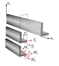 The internal forces in a beam are
quantified by internal force and moment vectors acting on each
cross-section. To make this precise,
introduce an imaginary cut perpendicular to the axis of the beam, as shown in the
figure. The stresses acting on an
interior face with normal parallel to the direction exert resultant forces T, and bending moments M. In an elastic beam with Youngs
modulus E and shear modulus , the bending moment vector is
related to the curvature vector by
The internal forces in a beam are
quantified by internal force and moment vectors acting on each
cross-section. To make this precise,
introduce an imaginary cut perpendicular to the axis of the beam, as shown in the
figure. The stresses acting on an
interior face with normal parallel to the direction exert resultant forces T, and bending moments M. In an elastic beam with Youngs
modulus E and shear modulus , the bending moment vector is
related to the curvature vector by
Here, may be replaced by a modified polar moment of
area to correct for warping of the cross-section.
For an
Euler-Bernoulli beam the force vector T is
a constraint (reaction) force and must be calculated using the equilibrium
equation. For a stretchable Timoshenko
beam the forces are related to the displacement of the neutral line and the
rotation vector by
where is a constant known as the ‘Timoshenko shear
coefficient’ for the beam. Since Timoshenko beam theory is (like all beam
theories) an approximation, the value of depends on how it is calculated. It depends on the geometry of the
cross-section and Poisson’s ratio, but for most practical applications one can
assume .
The static equilibrium equations for the internal forces are
As usual the finite element method
replaces these by the equivalent principle of virtual work. For a Timoshenko beam these are
For the Euler-Bernoulli beam the
components of T acting transverse to
the beam must be eliminated from the
virtual work equation, which gives
Here, and are kinematically admissible
variations in displacement and rotation, which must be related by the constraint
equation
Finite element method for elastic Euler-Bernoulli beams: There are three new features in the
virtual work equation for an Euler-Bernoulli beam:
1. The equation includes moments. These are related to the second derivative of
the displacements, or equivalently, the first derivative of the components of
the rotation vector. The appearance of
this second derivative means that the displacement and virtual displacement
field must be continuous for the finite element method to converge as the mesh
size is reduced.
2. The virtual work equation includes
the rotation vector;
3. The virtual work equation requires
that the rotation is correctly related to the displacement.
These new features mean that we must
use a special scheme to interpolate the displacement field. In fact, we solve not only for the
displacements, but also for the rotation, at discrete points along the beam.
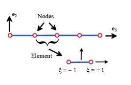 To this end, the beam is divided into
a series of elements bounded by nodes, as shown in the figure. The unknowns in the finite element solution
are the three components of displacement, and the three components of rotation,
at each node. We will set up a scheme
that allows these components to be expressed in an arbitrary basis (which allows the beam to have any
orientation in space), but for now, suppose that we wish to solve for their
components in the basis aligned with the beam.
To this end, the beam is divided into
a series of elements bounded by nodes, as shown in the figure. The unknowns in the finite element solution
are the three components of displacement, and the three components of rotation,
at each node. We will set up a scheme
that allows these components to be expressed in an arbitrary basis (which allows the beam to have any
orientation in space), but for now, suppose that we wish to solve for their
components in the basis aligned with the beam.
The axial displacement, and the axial
component of rotation (i.e. the twist) can then be interpolated linearly, since
these are differentiated only once in the virtual work equation. The transverse components of displacement
and rotation must be interpolated using cubic Hermitian polynomials, which
ensure that the rotation and displacement are continuous across neighboring
elements, and also that the rotation is correctly related to the
displacement. The interpolations can
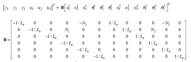
be conveniently written as a matrix expression
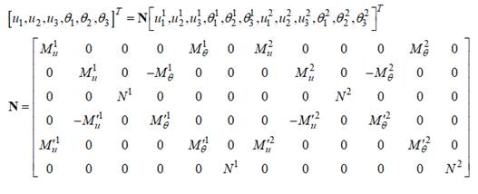
where and represent the displacements and rotations at
the two nodes of the element, and the interpolation functions are
with representing the normalized distance along the
element. The curvature and axial strain can then be computed as follows
where
The bending moment, twisting moment and axial force can then
be calculated as
Finally, in many applications
(particularly those involving several beams welded together to create a
structure) it is convenient to solve for displacement and rotation components
in a global basis, instead of using the components in the basis, which would differ for each beam. This can be accomplished by defining a basis
change matrix
where 0 represents a 3x3 null matrix, and represents the components of these vectors in
the global basis.
With these definitions, the principle of virtual work reduces
to a system of linear equations
where U is a vector of unknown nodal displacements and rotations (as
components in the basis), F
is a vector of nodal forces and moments, and
are the element stiffness matrix and force vector, with the coordinates and weights for a 2 point
Gauss integration scheme ( and ).
Finite element method for elastic Timoshenko beams: The principle of virtual work for the
Timoshenko beam consist of two coupled virtual work equations for the unknown
displacement and rotation of transverse cross-sections of the beam. The two are independent variables, so
1. There is no need to ensure that the
rotation are related by a compatibility constraint;
2. The displacement and rotation must be
continuous across element boundaries, but there is no need for continuity of
the derivative of the displacement.
This means that standard linear or
quadratic interpolation functions can be used to approximate their variations
within an element. Higher order
interpolation schemes can also be found in the literature.
To proceed with the finite element
formulation, it is helpful to combine the two virtual work equations for the
Timoshenko beam into a single, symmetric form.
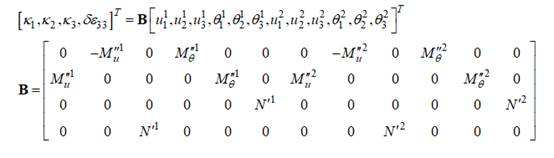
For this purpose we define a shear/axial strain vector
Adding the two virtual work equations then yields
This must hold for all admissible variations of .
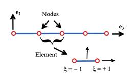 As before, the finite element version
of the virtual work principle is derived by dividing the beam into a series of
elements bounded by nodes, as shown in the figure. The unknowns in the finite element solution
are the three components of displacement, and the three components of rotation,
at each node that is adjacent to two neighboring elements. We will again set up
a scheme that allows the displacement and rotation components to be expressed
in an arbitrary basis (which allows the beam to have any
orientation in space), but begin by assuming that we wish to solve for their
components in the basis aligned with the beam.
As before, the finite element version
of the virtual work principle is derived by dividing the beam into a series of
elements bounded by nodes, as shown in the figure. The unknowns in the finite element solution
are the three components of displacement, and the three components of rotation,
at each node that is adjacent to two neighboring elements. We will again set up
a scheme that allows the displacement and rotation components to be expressed
in an arbitrary basis (which allows the beam to have any
orientation in space), but begin by assuming that we wish to solve for their
components in the basis aligned with the beam.
The displacement and rotation of the beam may be interpolated
linearly between the nodes as follows
Where
The curvature and shear/axial strain vectors can then be
calculated using
The internal forces and moments follow as
Finally, to re-write the finite
element equations in terms of displacement and rotation components in a global basis we once again define thebasis change
matrix
where 0 represents a 3x3 null matrix, and represents the components of these vectors in
the global basis.
With these definitions, the principle
of virtual work reduces to a system of linear equations
where U is a vector of unknown nodal displacements and rotations (as
components in the basis), F
is a vector of nodal forces and moments, and
are the element stiffness matrix and
force vector. The integrals have been
evaluated with a 1-point Gaussian quadrature scheme, in which the integrand is
calculated at , and the integration weight is .
A higher order integration scheme cannot be used, because it causes the
element to ‘lock,’ causing a spuriously high element stiffness matrix. This is particularly a problem in long,
slender beams with little shear deformation.
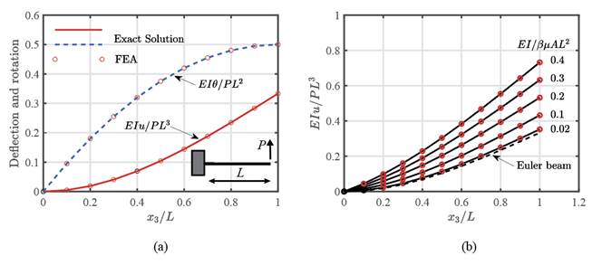
Example: A
simple demonstration of both the Euler-Bernoulli and Timoshenko beam elements
are shown in the figure. Fig. (a)
compares the predictions of the Euler-Bernoulli beam element for the deflection
and rotation of an end-loaded cantilever beam with the exact solution. The FEA predictions are within 0.1% of the
exact result with only 10 elements along the length of the beam. Fig. (b) shows the predicted deflection of
an end loaded Timoshenko beam, for several values of the normalized ratio of
bending to shear stiffness .
For the Timoshenko elements converge to the limit
of the Euler-Bernoulli beam. As shear deformation in the beam becomes
significant, and the Timoshenko elements predict a significantly larger
deflection than Euler-Bernoulli theory.
The codes that plot these graphs are provided in the files
named FEM_beam_Euler.m and FEM_beam_Timoshenko.m at
https://github.com/albower/Applied_Mechanics_of_Solids/
8.7.3 Plate Elements.
 We next consider simplified solid
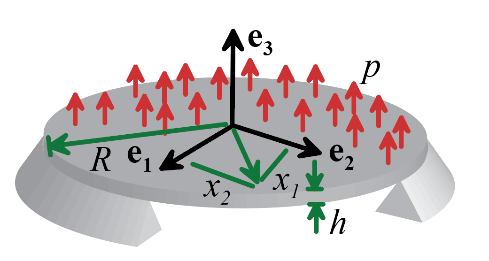
mechanics theories that describe motion of flat plates. The figure shows the problem to be
solved. Our goal is to calculate the
deflections and forces in a plate that is subjected to transverse forces on its
surface, and either supported or clamped on its edge, or subjected to in-plane
or transverse forces around its circumference.
To keep the discussion (reasonably) simple here, we will assume
We next consider simplified solid
mechanics theories that describe motion of flat plates. The figure shows the problem to be
solved. Our goal is to calculate the
deflections and forces in a plate that is subjected to transverse forces on its
surface, and either supported or clamped on its edge, or subjected to in-plane
or transverse forces around its circumference.
To keep the discussion (reasonably) simple here, we will assume
· The solid is a flat plate, with a uniform thickness h (in more sophistication FEA analysis,
plates can be curved - then they are called shells - and the thickness can vary)
· Deflections are
small, and the plate remains elastic.
· The plate is oriented so that the direction is normal to the undeformed
mid-section of the plate. In more
complex FEA simulations the plate may have an arbitrary orientation: in this
case the element stiffness matrices for the plate are first formulated using a
local coordinate system with normal to the plate, and then transformed to a
global coordinate frame. The procedure
was discussed in Section 8.7.2 for beams, but to keep things brief will not be
repeated in this section.
Summary of plate theory: Plate theory is discussed in (tedious) detail in Chapter 10,
but to understand how to solve the equations using the finite element method,
only a short summary is needed.
The deformed shape of a flat plate is
described by specifying the displacement of each point on the mid-section of the plate
as a function of position.
It is also necessary to calculate the
(small) rotation of the planes normal to the and directions in the undeformed plate. The rotation is quantified by a small
rotation vector , using one of two different
approaches:
1. Kirchhoff plate theory is an approximate theory (analogous to the Euler-Bernoulli
beam), which is intended to model plates that are thinner than 1/10th
of their in-plane dimensions. It assumes
that planes transverse to the mid-plane of the plate remain transverse after
deformation. In this case, the rotation
is related to the out-of-plane deflection of the plate by
These angles represent
the small rotation of a line that is transverse to the mid-plane of the
undeformed plate. They are components of
a vector, and are related to the transverse displacement by .
2. Reissner-Mindlin plate theory is a more complicated version, which allows the transverse
planes to rotate relative to the mid-plane of the plate. The rotation is then an independent
variable, which must be calculated as part of the solution.
In both theories, the curvature of the plate is defined as
The curvature is a (2D) tensor, and is related to the
rotation vector by
The strain distribution in the plate
is then
where the Greek indices have values 1 or 2.
The plate is in a state of plane stress, with internal
stresses
Reissner-Mindlin plate theory also
accounts approximately for the effects of the transverse shear stress
components , but these cannot be calculated
directly from the strain field
A plate may be loaded by subjecting
its edge to a force per unit length or moment per unit length. Alternatively, one or more components of
displacement or rotation may be prescribed.
In addition, a distributed force per unit area may act perpendicular to surface of the plate.
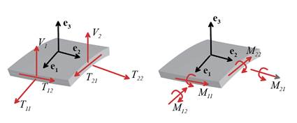
The forces in a plate are quantified
by internal force and moment tensors acting on each cross-section. To make this precise, cut a square element
from the plate with planes normal to the coordinate axes as shown in the
figure. A set of resultant forces and
moments act on the exposed faces:
· The moments are defined by
The physical significance of the
components is illustrated in the figure: characterizes the moment per unit length
acting on planes inside the shell that are normal to the direction, while characterizes the moment per unit length
acting on planes that are normal to .
Note that represents a moment about the axis, while is a moment acting about the axis. This can be expressed mathematically as where the repeated indices are summed over 1 and 2, but this expression
is only helpful if you are really good at visualizing dyadic and cross products.
· The in-plane forces are defined by
They represent resultant
forces exerted by stresses on the internal planes: are the components of force acting on the
plane perpendicular to the direction, while are those acting on the plane perpendicular to
the direction.
· The transverse forces represent forces acting in the direction on planes perpendicular to the and direction, respectively. In Kirchhoff theory they are constraint
forces and must be calculated from the equilibrium equation. In an exact version of Reissner-Mindlin
theory they would be related to the shear stresses acting on transverse planes
by
but the theory is approximate, so the
transverse forces are calculated instead through the rotation of the
cross-section, using the expressions given below.
The internal forces are related to the displacement and
curvature of the mid-plane of the plate by
In Reissner-Mindlin theory, the transverse shear forces are
related to the displacement and rotation by
where is a constant known as the ‘shear factor, ’
analogous to the shear coefficient for a beam.
Since the theory is approximate, the value of depends on how it is calculated. It depends on Poisson’s ratio, but for most
practical applications one can assume .
The static equilibrium equations for a plate are
This version of plate theory accounts
approximately for the effects of large in-plane loads on the out-of-plane
motion of the plate (so the theory can model a thin stretched membrane as well
as a plate). In simpler versions of plate
theory (which are more commonly used in practice) the terms involving products
of and in the moment equilibrium equation are
neglected.
For a finite element solution the equilibrium equations must
be re-cast as the equivalent principle of virtual work:
For the Kirchhoff plate, V
must be eliminated from the first two virtual work equations with the result
Finite element method for in-plane displacements and forces: In many practical applications the
in-plane displacements and forces in the plate may be neglected, but if needed,
they can be calculated before the out-of-plane displacements. Notice that the virtual work equation for the
in-plane displacements w and forces T decouple from those for the out-of-plane displacements and
rotations of the plate. Moreover, the
equation is identical (aside from the distinction between forces and stress) to
that for plane stress deformation of a plate.
Consequently, the equation can be solved using the procedure described
in Chapter 7, in which the in-plane displacement field is approximated by a linear
variation between the three nodes on the element. In this section we review the procedure
briefly, for convenience.
 A representative triangular plate
element is illustrated in the figure. It
has three nodes with coordinates , where k=1,2,3. Each node has two
in-plane displacement components , (the Greek indices have values 1 or
2), the out of plane displacement , and two rotation components .
A representative triangular plate
element is illustrated in the figure. It
has three nodes with coordinates , where k=1,2,3. Each node has two
in-plane displacement components , (the Greek indices have values 1 or
2), the out of plane displacement , and two rotation components .
The in-plane displacements and forces are then calculated as
follows:
1. Assemble the global stiffness matrix
and force vector
where the element stiffness and force
vector are
Here,
is the area of the element, is the length of a loaded element side, and the in-plane components of the (constant)
force per unit length acting on the side of the element, while
where
and
2. Modify the global stiffness to impose
any constraints on the in-plane displacements at the boundary
3. Solve the equation system for the in-plane displacements
4. Calculate the in-plane forces (which
are constant within each element) using , where is the 6 dimensional vector of the in-plane
displacements at the corners of the element.
Finite element method for out-of-plane deformation of elastic Kirchhoff
plates: We next
describe a method for calculating the out-of-plane deformation of a Kirchhoff
plate. The virtual work equation for the
out-of-plane motion resembles that for a beam, in that the equation involves
the curvature of the plate. This means
that ideally the out-of-plane displacements and its derivative must both be
continuous across the boundaries of an element. For a beam, it was possible to
find an interpolation scheme (using Hermitian polynomial shape functions) that
satisfied this condition exactly.
There is unfortunately no equivalent interpolation scheme for a
plate. Consequently, a large number of
different approaches to setting up interpolation schemes for plates have been
developed over the years, and new ones continue to appear. We will not attempt to review these here, and
instead will summarize how to set up a simple triangular plate element called
the ‘Specht triangle’ in honor of its author.
The out-of-plane motion of the plate
can be analyzed using the same mesh of triangular elements that is used to
model its in-plane motion. A
representative triangular plate element is illustrated in Fig 8.54. It has three nodes with coordinates , where k=1,2,3. Each node now has
an unknown out of plane displacement , and two rotation components .
As always, the goal is to calculate
the displacement and rotation at an arbitrary point within the element, given their values at the
three corner nodes with coordinates .
We define
where the interpolation functions are calculated as follows:
1. Calculate the ‘areal coordinates’ , where is the area of the triangle formed by a point
within the element and the two vertices opposite to node i, and is the area of the element:
2. Assemble a vector of products of
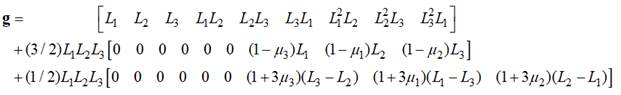
where
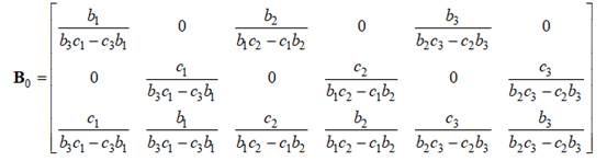
3. The shape functions can then be
calculated as weighted sums of the components of g:
where (as before)
4. The derivatives of the shape
functions are also needed: the first derivative can be calculated as
where
5. Similarly, the second derivatives are
Where
The curvature and rotation of the plate can then be
calculated as
where
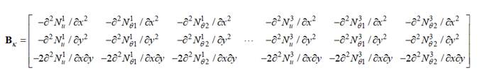
The bending moments follow as
where
With these definitions, the principle of virtual work reduces
to a system of linear equations
where U is a vector of unknown nodal displacements and rotations (as
components in the basis), F
is a vector of nodal forces and moments, and
are the element stiffness matrix and
force vector, with the coordinates for a 3 point Gauss
integration scheme
Finite element method for out-of-plane deformation of elastic
Reissner-Mindlin plates: The principle of virtual work for the
Reissner-Mindlin plate consists of two coupled virtual work equations for the
unknown displacement and rotation of transverse cross-sections of the
plate. The out of plane displacement
and the rotation of the plate are now two are independent variables,
1. There is no need to ensure that the
rotation are related by a compatibility constraint;
2. The displacement and rotation must be
continuous across element boundaries, but there is no need for continuity of
the derivative of the displacement.
At first sight this suggests that
displacements and rotations could be interpolated using the standard 2D shape
functions, but unfortunately these all suffer from shear locking if the plate
thickness is small. There have been many
attempts to design locking resistant plate elements. We will not attempt to review these here,
and instead describe the simple ‘Min3’ triangular element developed by Tessler
and Hughes as a representative example.
To proceed with the finite element formulation,
it is helpful to combine the two virtual work equations for the plate beam into
a single, symmetric form. For this
purpose we define a shear/axial strain vector
Adding the two virtual work equations then yields
As for the Kirchhoff plate, the
elements are triangular, such as the example illustrated in Fig 8.54. A generic element has three nodes with
coordinates , where k=1,2,3. Each node has an
unknown out of plane displacement , and two rotation components .
The displacement and rotation of the plate are now
interpolated separately as
where
with the areal coordinates
and
with
The derivatives of these shape functions can be calculated as
where
The displacement gradient, shear strain and curvatures are
related to the nodal displacements and rotations by
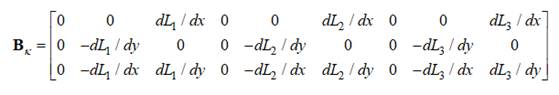
The internal forces follow as
With these definitions, the principle of virtual work reduces
to a system of linear equations
where U is a vector of unknown nodal displacements and rotations, F is a vector of nodal forces and
moments, and
are the element stiffness matrix and
force vector. The integrals have been
evaluated with a 3-point Gaussian quadrature scheme, with
A 1 point scheme will work as
well. The coefficient is a numerical correction that improves the
performance of the element. Tessler and
Hughes report that using
gives good results.
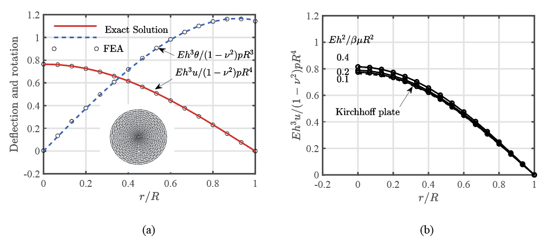
Example: A
simple demonstration of both the Kirchhoff and Reissner-Mindlin elements are
shown in the figure. Fig. (a) compares the predictions of the
Kirchhoff element for the deflection and rotation of a simply supported
circular plate with radius R, thickness
h,
Young’s modulus E, and Poisson’s
ratio subjected to uniform pressure p with the exact solution (the mesh is shown inset). The FEA predictions are within 0.1% of the
exact result. Fig. (b) shows the
predicted deflection of circular Reissner-Mindlin plate, for several values of
the normalized ratio of bending to shear stiffness .
The shear deformation increases the deflection slightly for >0.1 but the effect of shearing for the
circular plate is less pronounced than the corresponding behavior of a
cantilever beam discussed in the preceding section.
The codes that plot these graphs are provided in the files
named FEM_plate_Kirchhoff.m and FEM_plate_Mindlin.m at
https://github.com/albower/Applied_Mechanics_of_Solids/