8.6 Advanced element formulations $–$ Incompatible modes; reduced integration; B-bar and hybrid elements

 

Techniques for interpolating the displacement field within 2D and 3D finite elements were discussed in Section 8.1.9 and 8.1.10.  In addition, methods for evaluating the volume or area integrals in the principle of virtual work were discussed in Section 8.1.11.   These procedures work well for most applications, but there are situations where the simple element formulations can give very inaccurate results.  In this section

 

1. We illustrate some of the unexpected difficulties that can arise in apparently perfectly well designed finite element solutions to boundary value problems;

 

2. We describe a few more sophisticated elements that have been developed to solve these problems.

 

We focus in particular on `Locking’ phenomena.  Finite elements are said to `lock’ if they exhibit an unphysically stiff response to deformation.  Locking can occur for many different reasons. The most common causes are (i) the governing equations you are trying to solve are poorly conditioned, which leads to an ill conditioned system of finite element equations; (ii) the element interpolation functions are unable to approximate accurately the strain distribution in the solid, so the solution converges very slowly as the mesh size is reduced; (iii) in certain element formulations (especially beam, plate and shell elements) displacements and their derivatives are interpolated separately. Locking can occur in these elements if the interpolation functions for displacements and their derivatives are not consistent.

 

 

 

8.6.1 Shear locking and incompatible mode elements

 

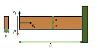
Shear locking can be illustrated by attempting to find a finite element solution to the simple boundary value problem illustrated in the figure. Consider a cantilever beam, with length L, height 2a and out-of-plane thickness b, as shown in the figure.  The top and bottom of the beam $x_2=\pm a$ are traction free, the left hand end is subjected to a resultant force P, and the right hand end is clamped.  Assume that b<<a, so that a state of plane stress is developed in the beam.  The analytical solution to this problem is given in Section 5.2.4.

 

The figure below compares this result to a finite element solution, obtained with standard 4 noded linear quadrilateral plane stress elements.  Results are shown for two different ratios of $a/L$. 

 

 

 

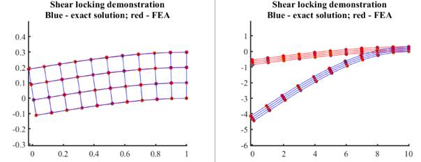
For a short, (or thick) beam, the finite element and exact solutions agree nearly perfectly.   For the long (or thin) beam, however, the finite element solution is very poor $–$ even though the mesh resolution is unchanged. The error in the finite element solution occurs because the standard 4 noded quadrilateral elements cannot accurately approximate the strain distribution associated with bending.  The phenomenon is known as ‘shear locking,’ because the element interpolation functions give rise to large, unphysical shear strains in bent elements, which makes them stiffer than they should be.  The solution would eventually converge if a large number of elements were added along the length of the beam. The elements would have to be roughly square, which would require about 133 elements along the length of the beam, giving a total mesh size of about 500 elements. 

 

Shear locking is therefore relatively benign, since it can be detected by refining the mesh, and can be avoided by using a sufficiently fine mesh.  However, finite element analysts sometimes cannot resist the temptation to reduce computational cost by using elongated elements, which can introduce errors.

 

Shear locking can also be avoided by using more sophisticated element interpolation functions that can accurately approximate bending. `Incompatible Mode’ elements do this by adding an additional strain distribution to the element.  The elements are called `incompatible’ because the strain is not required to be compatible with the displacement interpolation functions. The approach is conceptually straightforward:

 

1. The displacement fields in the element are interpolated using the standard scheme, by setting

$u_i={\displaystyle \sum _{a=1}^{N_e}{N}^a({\xi }_j)u_i^a}\delta v_i(x)={\displaystyle \sum _{a=1}^n{N}^a(x)\delta v_i^a}{x}_i={\displaystyle \sum _{a=1}^{N_e}{N}^a({\xi }_j)x_i^a}$ 

where $N^a({\xi }_j)$ are the shape functions listed in Sections 8.1.9 or 8.1.10, ${\xi }_i$ are a set of local coordinates in the element, $u_i^a,x_i^a$ denote the displacement values and coordinates of the nodes on the element, and $N_e$ is the number of nodes on the element.

 

2. The Jacobian matrix for the interpolation functions, its determinant, and its inverse are defined in the usual way

${\displaystyle \frac{\partial x_i}{\partial {\xi }_j}={\displaystyle \sum _{a=1}^{N_e}{\displaystyle \frac{\partial N^a(\xi )}{\partial {\xi }_j}{x}_i^a}}}$    $J=\det \left({\displaystyle \frac{\partial x_i}{\partial {\xi }_j}}\right)$        ${\displaystyle \frac{\partial {\xi }_j}{\partial x_i}={\left({\displaystyle \frac{\partial x}{\partial \xi }}\right)}_{ji}^{-1}}$

 

3. The usual expression for displacement gradient in the element is replaced by

${\displaystyle \frac{\partial u_i}{\partial x_j}=\left({\displaystyle \sum _{a=1}^{N_e}{\displaystyle \frac{\partial N^a(\xi )}{\partial {\xi }_m}}}{u}_i^a+{\displaystyle \sum _{k=1}^p{\displaystyle \frac{J(0)}{J(\xi )}}}{\alpha }_i^{(k)}{\delta }_{km}{\xi }_k\right){\displaystyle \frac{\partial {\xi }_m}{\partial x_j}}}$

where p=2 for a 2D problem and p=3 for a 3D problem, ${\alpha }_i^{(k)}$ are a set of unknown displacement gradients in the element, which must be determined as part of the solution.

 

4. Similarly, the virtual displacement gradient is written as

${\displaystyle \frac{\partial \delta v_i}{\partial x_j}=\left({\displaystyle \sum _{a=1}^{N_e}{\displaystyle \frac{\partial N^a(\xi )}{\partial {\xi }_m}}}\delta v_i^a+{\displaystyle \sum _{k=1}^p{\displaystyle \frac{J(0)}{J(\xi )}}}\delta {\alpha }_i^{(k)}{\delta }_{km}{\xi }_k\right){\displaystyle \frac{\partial {\xi }_m}{\partial x_j}}}$

where $\delta {\alpha }_i^{(k)}$ is a variation in the internal displacement gradient field for the element.  

 

5. These expressions are then substituted into the virtual work equation, which must now be satisfied for all possible values of virtual nodal displacements $\delta v_i^a$ and virtual displacement gradients $\delta {\alpha }_i^{(k)}$.  At first sight this procedure appears to greatly increase the size of the global stiffness matrix, because a set of unknown displacement gradient components must be calculated for each element.  However, the unknown ${\alpha }_i^{(k)}$ are local to each element, and can be eliminated while computing the element stiffness matrix. 

 

 

As always actual computations are best accomplished by re-writing the calculations as matrix operations.   We will illustrate the procedure using 2D (plane stress or strain) elements as an example; the modification to 3D is straightforward.   The calculation follows the steps in Section 8.1.13, but the matrix B is replaced by one that maps displacements and the additional element degrees of freedom onto the strain vector, as $\epsilon =B{[u,\alpha ]}^T$, where

$\epsilon ={[{\epsilon }_{11},{\epsilon }_{22},2{\epsilon }_{12}]}^{T}u=\left[u_1^1,u_2^1,u_1^2,u_2^2\mathrm{...}\right]\alpha =\left[{\alpha }_1^1,{\alpha }_2^1,{\alpha }_1^2,{\alpha }_2^2\mathrm{...}\right]$

$B=\left[\begin{array}{cccccc}{\displaystyle \frac{\partial N^1}{\partial x_1}}& 0& {\displaystyle \frac{\partial N^2}{\partial x_1}}& 0& {\displaystyle \frac{\partial N^3}{\partial x_1}}& 0\\ 0& {\displaystyle \frac{\partial N^1}{\partial x_2}}& 0& {\displaystyle \frac{\partial N^2}{\partial x_2}}& 0& {\displaystyle \frac{\partial N^3}{\partial x_2}}\\ {\displaystyle \frac{\partial N^1}{\partial x_2}}& {\displaystyle \frac{\partial N^1}{\partial x_1}}& {\displaystyle \frac{\partial N^2}{\partial x_2}}& {\displaystyle \frac{\partial N^2}{\partial x_1}}& {\displaystyle \frac{\partial N^3}{\partial x_2}}& {\displaystyle \frac{\partial N^3}{\partial x_1}}\end{array}\mathrm{.......}\begin{array}{cccc}{\displaystyle \frac{J(0)}{J(\xi )}{\xi }_1{\displaystyle \frac{\partial {\xi }_1}{\partial x_1}}}& 0& {\displaystyle \frac{J(0)}{J(\xi )}{\xi }_2{\displaystyle \frac{\partial {\xi }_2}{\partial x_1}}}& 0\\ 0& {\displaystyle \frac{J(0)}{J(\xi )}{\xi }_1{\displaystyle \frac{\partial {\xi }_1}{\partial x_2}}}& 0& {\displaystyle \frac{J(0)}{J(\xi )}{\xi }_2{\displaystyle \frac{\partial {\xi }_2}{\partial x_2}}}\\ {\displaystyle \frac{J(0)}{J(\xi )}{\xi }_1{\displaystyle \frac{\partial {\xi }_1}{\partial x_2}}}& {\displaystyle \frac{J(0)}{J(\xi )}{\xi }_1{\displaystyle \frac{\partial {\xi }_1}{\partial x_1}}}& {\displaystyle \frac{J(0)}{J(\xi )}{\xi }_2{\displaystyle \frac{\partial {\xi }_2}{\partial x_2}}}& {\displaystyle \frac{J(0)}{J(\xi )}{\xi }_2{\displaystyle \frac{\partial {\xi }_2}{\partial x_1}}}\end{array}\right]$

The standard procedure is then used to calculate an intermediate stiffness matrix that includes additional rows and columns arising from the incompatible modes

$\widehat{k}={\displaystyle \sum _{I=1}^{N_i}{B}^{T}DBJ{w}_I}\widehat{r}={\displaystyle \sum _{I=1}^{N_i}{B}^T\sigma J{w}_I}$

These matrices relate the degrees of freedom on the element by

$\left[\begin{array}{cc}{k}^{uu}& k^{u\alpha }\\ k^{\alpha u}& k^{\alpha \alpha }\end{array}\right]\left[\begin{array}{c}u\\ \alpha \end{array}\right]=\left[\begin{array}{c}{r}^u\\ r^{\alpha }\end{array}\right]$

where $k^{uu}$ is a (2nx2n) matrix, with n the number of nodes on the element and $k^{\alpha \alpha }$ is a 4x4 matrix.   We can use the last four rows to eliminate $\alpha$, with the result

$\left[k^{uu}-k^{u\alpha }{k}^{\alpha \alpha -1}{k}^{\alpha u}\right]u=r^u-k^{\alpha \alpha -1}{r}^{\alpha }$

The usual 2nx2n element stiffness matrix (which only has displacements as degrees of freedom) and residual force are therefore

$\begin{array}{l}{k}^{el}=\left[k^{uu}-k^{u\alpha }{k}^{\alpha \alpha -1}{k}^{\alpha u}\right]u=\\ r^{el}=r^u-k^{\alpha \alpha -1}{r}^{\alpha }\end{array}$

 

A sample small-strain, linear elastic code with incompatible mode elements Femlinelast_incompatible_modes.m can be downloaded from https://github.com/albower/Applied_Mechanics_of_Solids .

 

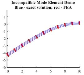
When run with the input file shear_locking_demo.txt, the codes produce the results shown in the figure below.  The incompatible modes clearly give a spectacular improvement in the performance of the element.

 

 

 

HEALTH WARNINGS: (i) The procedure outlined here only works for small-strain problems.  Finite strain versions exist but are somewhat more complicated.  (ii)  Adding strain variables to elements can dramatically improve their performance, but this procedure must be used with great care to ensure that the strain and displacement degrees of freedom are independent variables. For further details see Simo,  J. C., and M. S. Rifai, Int J. Num. Meth in Eng.  29, pp. 1595$–$1638, 1990. Simo,  J. C., and F. Armero, Int J. Num. Meth in Eng., 33, pp. 1413$–$1449, 1992.

 

 

 

8.6.2 Volumetric locking and reduced integration elements

 

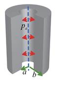
Volumetric locking can be illustrated using a simple boundary value problem. Consider a long hollow cylinder with internal radius a and external radius b as shown in the figure.   The solid is made from a linear elastic material with Young’s modulus $E$ and Poisson’s ratio $\nu$.  The cylinder is loaded by an internal pressure $p_a$ and deforms in plane strain.  The analytical solution to this problem is given in Section 4.1.9.

 

The figure below compares the analytical solution to a finite element solution with standard 4 noded plane strain quadrilateral elements.  Results are shown for two values of Poisson’s ratio $\nu$.  The dashed lines show the analytical solution, while the solid line shows the FEA solution.

 

 

           

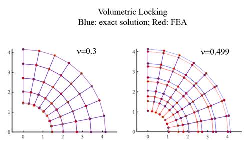
The two solutions agree well for $\nu =0.3$, but the finite element solution grossly underestimates the displacements as Poisson’s ratio is increased towards 0.5 (recall that the material is incompressible in the limit $\nu =0.5$ ).  In this limit, the finite element displacements tend to zero $–$ this is known as `volumetric locking’

 

The error in the finite element solution occurs because the finite element interpolation functions are unable to properly approximate a volume preserving strain field. In the incompressible limit, a nonzero volumetric strain at any of the integration points gives rise to a very large contribution to the virtual power.  The interpolation functions can make the volumetric strain vanish at some, but not all, the integration points in the element. 

 

Volumetric locking is a much more serious problem than shear locking, because it cannot be avoided by refining the mesh.  In addition, all the standard fully integrated finite elements will lock in the incompressible limit; and some elements show very poor performance even for Poisson’s ratios as small as $0.45$.  Fortunately, most materials have Poisson’s ratios around 0.3 or less, so the standard elements can be used for most linear elasticity and small-strain plasticity problems.   To model rubbers, or to solve problems involving large plastic strains, the elements must be redesigned to avoid locking.

 

 

Reduced Integration is the simplest way to avoid locking.   The basic idea is simple: since the fully integrated elements cannot make the strain field volume preserving at all the integration points, it is tempting to reduce the number of integration points so that the constraint can be met.  `Reduced integration’ usually means that the element stiffness is integrated using an integration scheme that is one order less accurate than the standard scheme.   The number of reduced integration points for various element types is listed in Table 8.11.  The coordinates of the integration points are listed in the tables in Section 8.1.12.

 

HEALTH WARNING: Notice that the integration order cannot be reduced for the linear triangular and tetrahedral elements $–$ these elements should not be used to model near incompressible materials, although in desperation you can a few such elements in regions where the solid cannot be meshed using quadrilaterals.

 

Remarkably, reduced integration completely resolves locking in some elements (the quadratic quadrilateral and brick), and even improves the accuracy of the element.  As an example, the leftmost figure below  shows the solution to the pressurized cylinder problem, using reduced integration (with 4 integration points) for 8 noded quadrilaterals.  With reduced integration, the analytical and finite element results are indistinguishable.

 

 

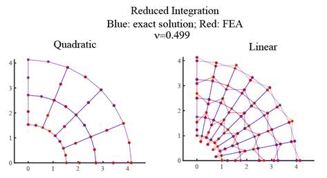
Reduced integration does not work in 4 noded quadrilateral elements or 8 noded brick elements.  For example, the right hand figure above  shows the solution to the pressure vessel problem with linear (4 noded) quadrilateral elements with reduced integration (1 integration point).  The displacements have been scaled down to show the hourglassing $–$ plotted to true scale the displacements just look like complete garbage.  The solution is clearly a disaster.  The error occurs because the stiffness matrix is nearly singular $–$  the system of equations includes a weakly constrained deformation mode. This   phenomenon is known as ‘hourglassing’ because of the characteristic shape of the spurious deformation mode. 

 

 

Selectively Reduced Integration can be used to cure hourglassing.   The procedure is illustrated most clearly by modifying the formulation for static linear elasticity. To implement the method: 

 

1. The volume integral in the virtual work principle is separated into a deviatoric and volumetric part by writing

${\displaystyle \underset{R}{\int }{\sigma }_{ij}\delta {\epsilon }_{ij}d{V}_0}={\displaystyle \underset{R}{\int }\left({\sigma }_{ij}\delta {\epsilon }_{ij}-{\displaystyle \frac{{\sigma }_{kk}}{3}\delta {\epsilon }_{qq}}\right)d{V}_0}+{\displaystyle \underset{R}{\int }{\displaystyle \frac{{\sigma }_{kk}}{3}\delta {\epsilon }_{qq}d{V}_0}}$

 Here, the first integral on the right hand side vanishes for a hydrostatic stress.

 

2. Substituting the linear elastic constitutive equation and the finite element interpolation functions into the virtual work principle, we find that the element stiffness matrix can be reduced to

$k_{aibk}^{(l)}={\displaystyle \underset{V_e^{(l)}}{\int }\left(C_{ijkl}{\displaystyle \frac{\partial N^a(x)}{\partial x_j}{\displaystyle \frac{\partial N^b(x)}{\partial x_l}-{\displaystyle \frac{1}{3}{C}_{ppkl}{\displaystyle \frac{\partial N^a(x)}{\partial x_i}{\displaystyle \frac{\partial N^b(x)}{\partial x_l}}}}}}\right)dV}+{\displaystyle \underset{V_e^{(l)}}{\int }{\displaystyle \frac{1}{3}{C}_{ppkl}{\displaystyle \frac{\partial N^a(x)}{\partial x_i}{\displaystyle \frac{\partial N^b(x)}{\partial x_l}dV}}}}$

 

3. When selectively reduced integration is used, the first volume integral is evaluated using the full integration scheme; the second integral is evaluated using reduced integration points.  The matrix form of the formula for the stiffness can be written as

$k_{el}={\displaystyle \sum _{I=1}^{N_i}{B}^T{D}^{Dev}BJ{w}_I}+{\displaystyle \sum _{I=1}^{M_i}{B}^T{D}^{Vol}BJ{w}_I}$

where $N_i,M_i$ denote the numbers of full and reduced integration points, respectively, and the matrices of elastic constants (for an isotropic material in 3D) are

$D^{Dev}={\displaystyle \frac{E}{(1+\nu )}\left[\begin{array}{cccccc}2/3& -1/3& -1/3& 0& 0& 0\\ -1/3& 2/3& -1/3& 0& 0& 0\\ -1/3& -1/3& 2/3& 0& 0& 0\\ 0& 0& 0& 1/2& 0& 0\\ 0& 0& 0& 0& 1/2& 0\\ 0& 0& 0& 0& 0& 1/2\end{array}\right]}$

$D^{Vol}={\displaystyle \frac{E}{3(1-2\nu )}\left[\begin{array}{cccccc}1& 1& 1& 0& 0& 0\\ 1& 1& 1& 0& 0& 0\\ 1& 1& 1& 0& 0& 0\\ 0& 0& 0& 0& 0& 0\\ 0& 0& 0& 0& 0& 0\\ 0& 0& 0& 0& 0& 0\end{array}\right]}$

 

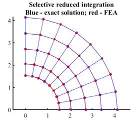
Selective reduced integration has been implemented in the sample Matlab code Fem_selective_reduced_integration.m. The code can be downloaded from

https://github.com/albower/Applied_Mechanics_of_Solids .

 

When this code is run with the input file volumetric_locking_demo.txt it produces the results shown in the figure below.   The analytical and finite element solutions agree, and there are no signs of hourglassing.

 

 

 

 

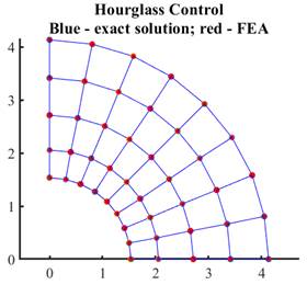
Reduced integration with hourglass control: Hourglassing in 4 noded quadrilateral and 8 noded brick elements can also be cured by adding an artificial stiffness to the element that acts to constrain the hourglass mode.   The stiffness must be carefully chosen so as to influence only the hourglass mode.  Only the final result will be given here $–$ for details see D.P. Flanagan and T. Belytschko, (1981).  To compute the corrective term:

 

1. Define a series of ‘hourglass base vectors’  ${\Gamma }^{a(i)}$ which specify the displacements of the ath node in the ith hourglass mode.   The 4 noded quadrilateral element has only one hourglass mode; the 8 noded brick has 4 modes, listed in the table.

 

2. Calculate the `hourglass shape vectors’ for each mode as follows

${\gamma }^{a(i)}={\Gamma }^{a(i)}-{\displaystyle \frac{\partial N^a(\xi =0)}{\partial x_j}{\displaystyle \sum _{b=1}^{n_e}{\Gamma }^{b(i)}{x}_j^b}}$

where $n_e$ denotes the number of nodes on the element.

 

3. The modified stiffness matrix for the element is written as

$k_{aibk}^{(l)}={\displaystyle \underset{V_e^{(l)}}{\int }{C}_{ijkl}{\displaystyle \frac{\partial N^a(x)}{\partial x_j}{\displaystyle \frac{\partial N^b(x)}{\partial x_l}dV}}}+\kappa V_e^{(l)}{\displaystyle \sum _m{\gamma }^{a(m)}{\gamma }^{b(m)}}$

where $V_e$ denotes the volume of the element, and $\kappa$ is a numerical parameter that controls the stiffness of the hourglass resistance.  Taking $\kappa =0.01\mu \left(\partial N^a/\partial x_j\right)\left(\partial N^a/\partial x_j\right)$ where $\mu$ is the elastic shear modulus works well for most applications.  If $\kappa$ is too large, it will seriously over-stiffen the solid.

 

 

Sample code: Reduced integration with hourglass control has been implemented in the sample Matlab code Fem_hourglasscontrol.m.   When run with the input file volumetric_locking_demo.txt it produces the results shown in the figure below. Hourglassing has clearly been satisfactorily eliminated.

 

 

 

 

HEALTH WARNING: Hourglass control is not completely effective: it can fail for finite strain problems and can also cause problems in a dynamic analysis, where the low stiffness of the hourglass modes can introduce spurious low frequency vibration modes and low wave speeds.

 

 

 

8.6.3 Volumetric locking and ‘B-bar’ elements

 

The ‘B-bar’ method for small strains:  Like selective reduced integration, the B-bar method works by treating the volumetric and deviatoric parts of the stiffness matrix separately.  Instead of separating the volume integral into two parts, however, the B-bar method modifies the definition of the strain in the element.  Its main advantage is that the concept can easily be generalized to finite strain problems.   Here, we will illustrate the method by applying it to small-strain linear elasticity.  The procedure starts with the usual virtual work principle 

${\displaystyle \underset{R}{\int }{\sigma }_{ij}[{\epsilon }_{ij}(u_k)]\delta {\epsilon }_{ij}dV-{\displaystyle \underset{R}{\int }{b}_i\delta v_{i}dV-{\displaystyle \underset{{\partial }_{2}R}{\int }{t}_i^{*}\delta v_{i}dA=0}}}$

In the B-bar method

1. We introduce a new variable to characterize the volumetric strain in the elements.  Define

$\omega ={\displaystyle \frac{1}{3V_e}{\displaystyle \underset{V_e}{\int }{\epsilon }_{kk}dV}}$

where the integral is taken over the volume of the element.

 

2. The strain in each element is replaced by the approximation ${\overline{\epsilon }}_{ij}={\epsilon }_{ij}+(\omega -{\epsilon }_{kk}/3){\delta }_{ij}$

 

3. Similarly, the virtual strain in each element is replaced by $\delta {\overline{\epsilon }}_{ij}=\delta {\epsilon }_{ij}+(\delta \omega -\delta {\epsilon }_{kk}/3){\delta }_{ij}$

 

This means that the volumetric strain in the element is everywhere equal to its mean value.  The virtual work principle is then written in terms of ${\overline{\epsilon }}_{ij}$ and $\delta {\overline{\epsilon }}_{ij}$ as

${\displaystyle \underset{R}{\int }{\sigma }_{ij}[{\overline{\epsilon }}_{ij}(u_k)]\delta {\overline{\epsilon }}_{ij}dV-{\displaystyle \underset{R}{\int }{b}_i\delta v_{i}dV-{\displaystyle \underset{{\partial }_{2}R}{\int }{t}_i^{*}\delta v_{i}dA=0}}}$

Finally, introducing the finite element interpolation and using the constitutive equation yields the usual system of linear finite element equations, but with a modified element stiffness matrix (and for nonlinear problems, a modified residual force vector).    The stiffness and element residual are assembled using the steps outlined in Section 8.1.13, but with the following modifications:

 

1. Before calculating the stiffness matrix, the volume average of the shape function derivatives must be computed.   This means an additional loop over the integration points, calculating the spatial shape function derivatives at each successive integration point (as in Step 1 of 8.1.13) and assembling the sums

$V_{el}={\displaystyle \sum _{I=1}^{N_I}J{w}_I}H={\displaystyle \sum _{I=1}^{N_I}{\displaystyle \frac{dN}{dx}J{w}_I}}$

A reduced integration scheme is usually sufficient.   Once the sum has been computed the volume average shape function derivatives follow as

$\overline{{\displaystyle \frac{dN}{dx}}}={\displaystyle \frac{H}{V_{el}}}$

 

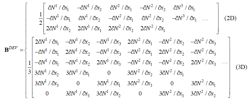
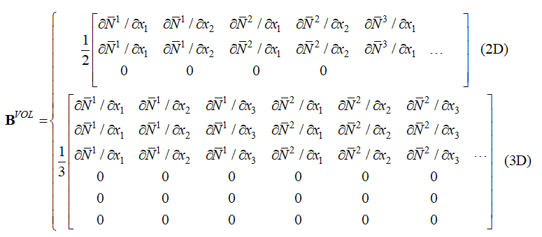
2. The element stiffness matrix and residual force vector are then assembled as before, except that the strain vector and B matrix are modified to

$\overline{\epsilon }=BU$

with

$\overline{\epsilon }=\left\{\begin{array}{c}{\left[\begin{array}{ccc}{\overline{\epsilon }}_{11}& {\overline{\epsilon }}_{22}& 2{\overline{\epsilon }}_{12}\end{array}\right]}^T(2\text{D)}\\ {\left[\begin{array}{cccccc}{\overline{\epsilon }}_{11}& {\overline{\epsilon }}_{22}& {\overline{\epsilon }}_{33}& 2{\overline{\epsilon }}_{12}& 2{\overline{\epsilon }}_{13}& 2{\overline{\epsilon }}_{23}\end{array}\right]}^T(3\text{D)}\end{array}\right.$

$\overline{B}=B^{DEV}+B^{VOL}$

 

The stress follows as $\sigma =D\overline{\epsilon }$ and the element stiffness and residual force are calculated using the usual expressions

$k_{el}={\displaystyle \sum _{I=1}^{N_i}{\overline{B}}^{T}D\overline{B}J{w}_I}{r}_{el}={\displaystyle \sum _{I=1}^{N_i}{\overline{B}}^T\sigma J{w}_I}$

The sums can be evaluated using a standard, full integration scheme.

 

The B-bar method for small strains has been implemented in the sample code or FEM_Bbar.m.  The code can be run with the input file volumetric_locking_demo.txt.  Run the code yourself to verify that the analytical and finite element solutions agree, and there are no signs of hourglassing.

 

The ‘B-bar’ method for large strains:  The B-bar method can also be extended to finite deformations.   As a representative application, we will use it to solve the problem involving deformation of a hyperelastic material that was discussed in Section 8.4.   Most hyperelastic materials have a large bulk modulus compared to their shear modulus (and are often idealized as incompressible materials).   As we have seen, it is important to design elements carefully for this sort of material.  The simple implementation described Section 8.4 will suffer from volumetric locking. The approach discussed below will resolve this problem.

As in the small strain B-bar method the basic idea is to interpolate the volumetric and deviatoric strains separately.   In finite strain problems we use the deformation gradient as the basic measure of deformation rather than the strain; as you probably know, the Jacobian of the deformation gradient quantifies volume changes.   Accordingly, the B-bar method for finite strains uses a modified measure of the Jacobian of the deformation gradient.  To this end:

 

1. We define the volume averaged Jacobian of the deformation gradient

$\eta ={\displaystyle \frac{1}{V_{el}}{\displaystyle \underset{V_{el}}{\int }\det (F)dV}}$

Here, the integral is taken over the volume of the element in the reference configuration.

 

2. The deformation gradient is replaced by an approximation ${\overline{F}}_{ij}=F_{ij}{\left(\eta /J\right)}^{1/n}$, where n=2 for a 2D plane strain problem and n=3 for a 3D problem, while J=det(F).

 

3. The virtual work equation is expressed in terms of this modified deformation gradient as

                                             ${\displaystyle \underset{R_0}{\int }{\tau }_{ij}[{\overline{F}}_{kl}]\delta {\overline{L}}_{ij}d{V}_0-{\displaystyle \underset{R_0}{\int }{\rho }_0{b}_i\delta v_{i}d{V}_0-{\displaystyle \underset{{\partial }_2{R}_0}{\int }{t}_i^{*}\delta v_i\eta d{A}_0}=0}}$ 

where ${\tau }_{ij}=J{\sigma }_{ij}$ is the Kirchhoff stress,

$\delta {\overline{L}}_{ij}=\delta {\dot{\overline{F}}}_{ik}{\overline{F}}_{kj}^{-1}=\delta L_{ij}+{\displaystyle \frac{{\delta }_{ij}}{n}\left({\displaystyle \frac{\delta \dot{\eta }}{\eta }-\delta L_{kk}}\right)}$

and

$\delta \dot{\eta }={\displaystyle \frac{1}{V_{el}}{\displaystyle \underset{V_{el}}{\int }J{F}_{ji}^{-1}\delta {\dot{F}}_{ij}dV}={\displaystyle \frac{1}{V_{el}}{\displaystyle \underset{V_{el}}{\int }J\delta L_{kk}dV}}}$

 

4. We now introduce the usual element interpolation functions and calculate the deformation gradient and velocity gradient as

$\begin{array}{l}{F}_{ij}={\delta }_{ij}+{\displaystyle \frac{\partial u_i}{\partial x_j}={\delta }_{ij}+{\displaystyle \sum _{a=1}^n{\displaystyle \frac{\partial N^a}{\partial x_j}{u}_i^a}}}\\ \delta L_{ij}={\displaystyle \frac{\partial \delta v_i}{\partial y_j}={\displaystyle \sum _{a=1}^n{\displaystyle \frac{\partial N^a}{\partial y_j}\delta v_i^a}}{\displaystyle \frac{\partial N^a}{\partial y_j}={\displaystyle \frac{\partial N^a}{\partial x_k}{F}_{kj}^{-1}}}}\end{array}$

 

5. As in the small-strain B-bar method we introduce the volume averaged shape function derivatives

$\overline{{\displaystyle \frac{\partial N^a}{\partial y_i}}}={\displaystyle \frac{1}{\eta V_{el}}{\displaystyle \underset{V_{el}}{\int }J{\displaystyle \frac{\partial N^a}{\partial y_i}dV}}}$

 

6. With these identities the discrete equilibrium equation can be expressed as

$\begin{array}{l}{R}_i^a-F_i^a=0\\ F_i^a={\displaystyle \underset{R_0}{\int }{\rho }_0{b}_i{N}^{a}d{V}_0+{\displaystyle \underset{{\partial }_2{R}_0}{\int }{t}_i^{*}{N}^a\widehat{\eta }d{A}_0}}\\ R_i^a={\displaystyle \underset{R_0}{\int }{\tau }_{mj}[{\overline{F}}_{kl}]\left[{\delta }_{im}{\displaystyle \frac{\partial N^a}{\partial y_j}+{\displaystyle \frac{{\delta }_{mj}}{n}\left(\overline{{\displaystyle \frac{\partial N^a}{\partial y_i}}}-{\displaystyle \frac{\partial N^a}{\partial y_i}}\right)}}\right]d{V}_0}\end{array}$

 

7. The equilibrium equation is nonlinear, and must be solved using Newton-Raphson iteration. This means repeatedly solving

$K_{aibk}^{}d{w}_k^b=-R_i^a+F_i^a$

 

for the correction $d{w}_k^b$ to the current approximation to the displacement field.  The stiffness follows from linearizing the virtual work equation.  The resulting element stiffness is

$\begin{array}{l}{k}_{aibk}^{el}={\displaystyle \underset{R_0}{\int }\left({\delta }_{im}{\displaystyle \frac{\partial N^a}{\partial y_j}+{\displaystyle \frac{{\delta }_{mj}}{n}\left(\overline{{\displaystyle \frac{\partial N^a}{\partial y_i}}}-{\displaystyle \frac{\partial N^a}{\partial y_i}}\right)}}\right){\displaystyle \frac{\partial {\tau }_{mj}[B_{kl}]}{\partial B_{ln}}{\displaystyle \frac{\partial B_{ln}}{\partial {\overline{F}}_{ps}}{\overline{F}}_{rs}\left({\displaystyle \frac{\partial N^b}{\partial y_r}{\delta }_{pk}+{\displaystyle \frac{{\delta }_{pr}}{n}\left(\overline{{\displaystyle \frac{\partial N^b}{\partial y_k}}}-{\displaystyle \frac{\partial N^b}{\partial y_k}}\right)}}\right)d{V}_0}}}\\ +{\displaystyle \underset{R_0}{\int }-{\tau }_{ij}[B_{kl}]{\displaystyle \frac{\partial N^a}{\partial y_k}{\displaystyle \frac{\partial N^b}{\partial y_j}+{\tau }_{jj}[{\overline{F}}_{kl}]{\displaystyle \frac{1}{n}\left(Q_{aibk}+{\displaystyle \frac{\partial N^a}{\partial y_k}{\displaystyle \frac{\partial N^b}{\partial y_i}-\overline{{\displaystyle \frac{\partial N^a}{\partial y_i}}}\overline{{\displaystyle \frac{\partial N^b}{\partial y_k}}}}}\right)d{V}_0}}}}\end{array}$

where

$Q_{aibk}={\displaystyle \frac{1}{\eta V_{el}}{\displaystyle \underset{V_{el}}{\int }\left(J{\displaystyle \frac{\partial N^b}{\partial y_k}{\displaystyle \frac{\partial N^a}{\partial y_i}-J{\displaystyle \frac{\partial N^a}{\partial y_k}{\displaystyle \frac{\partial N^b}{\partial y_i}}}}}\right)dV}}$

 

8. The element residual force and stiffness can be re-written as matrix operations as follows:

$\begin{array}{l}{r}_{el}={\displaystyle \sum _{I=1}^{N_i}{\overline{A}}^T\tau \widehat{J}{w}_I}\\ k_{el}={\displaystyle \sum _{I=1}^{N_i}\left({\overline{A}}^{T}DG{\overline{A}}^{*}-P\odot S+{\displaystyle \frac{{\tau }_{jj}}{n}\left\{Q+P\odot P^T-\overline{\nu }\otimes \overline{\nu }\right\}}\right)\widehat{J}{w}_I}\\ Q={\displaystyle \frac{1}{\eta V_{el}}{\displaystyle \sum _{I=1}^{N_i}J\left(\nu \otimes \nu -P\odot P^T\right)\widehat{J}{w}_I}}\end{array}$

where (for a 3D problem)

 

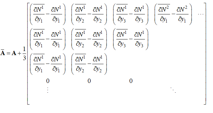
where $A,A^{*}$ as well as $P,S$ are the matrices of shape function derivatives defined in Section 8.4.6, except that for finite strain problems $dN/dx$ in 8.4.6 must be replaced by $dN/dy=(dN/dx)F^{-1}$. Similarly, matrices D and G are defined in 8.4.6, but must be calculated using the modified deformation gradient $\overline{F}$.   Finally

$\nu =\left[\begin{array}{ccccccc}{\displaystyle \frac{\partial N^1}{\partial y_1}}& {\displaystyle \frac{\partial N^1}{\partial y_2}}& {\displaystyle \frac{\partial N^1}{\partial y_3}}& {\displaystyle \frac{\partial N^2}{\partial y_1}}& {\displaystyle \frac{\partial N^2}{\partial y_2}}& {\displaystyle \frac{\partial N^2}{\partial y_3}}& \cdots \end{array}\right]$

is a vector of shape function derivatives, and $\overline{\nu }$ is the same quantity with $\partial N/\partial y$ replaced by $\overline{\partial N}/\partial y$.  The integrals may be evaluated with a full integration scheme.

 

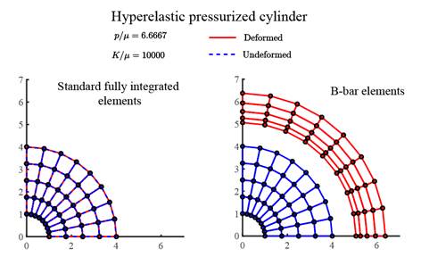
Sample Code: The B-bar method for finite strains has been implemented in the sample code or FEM_bbar_hyperelastic.m.  The code can be run with the input file bbar_hypere_demo.txt.  The file calculates the deformation of a long hollow cylinder with internal radius a and external radius b=4a as shown in the figure below.  The solid is made from a modified neo-hookean material described in Section 3.5 (see also Section 8.4), with shear modulus $\mu$ modulus  and bulk modulus $K$.  The cylinder is loaded by an internal pressure $p$  and deforms in plane strain.  The predicted deformation of the cylinder is shown in the figure below.  Results on the right were obtained with the B-bar elements described in this section; while those on the left were obtained with the standard fully integrated isoparametric elements described in Section 8.4.   The figure confirms that the B-bar element successfully cures locking in the standard formulation.

 

 

 

 

 

8.6.4 Hybrid elements for modeling near-incompressible materials

 

The bulk elastic modulus is infinite for a fully incompressible material, which leads to an infinite stiffness matrix in the standard finite element formulation (even if reduced integration is used to avoid locking).   This behavior can cause the stiffness matrix for a nearly incompressible material to become ill-conditioned, so that small rounding errors during the computation result in large errors in the solution.

 

Hybrid elements are designed to avoid this problem.  They work by including the hydrostatic stress distribution as an additional unknown variable, which must be computed at the same time as the displacement field.  This allows the stiff terms to be removed from the system of finite element equations.  The procedure is illustrated most easily using isotropic linear elasticity, but in practice hybrid elements are usually used to simulate rubbers or metals subjected to large plastic strains.

 

Hybrid elements are based on a modified version of the principle of virtual work, as follows. The virtual work equation (for small strains) is re-written as

${\displaystyle \underset{R}{\int }\left(S_{ij}\delta {\epsilon }_{ij}\right)d{V}_0}+{\displaystyle \underset{R}{\int }p\delta {\epsilon }_{qq}d{V}_0}+{\displaystyle \underset{R}{\int }\delta p\left({\displaystyle \frac{{\sigma }_{kk}}{3K}-{\displaystyle \frac{p}{K}}}\right)d{V}_0}-{\displaystyle \underset{R}{\int }{b}_i\delta v_{i}d{V}_0-{\displaystyle \underset{{\partial }_{2}R}{\int }{t}_i\delta v_{i}dA}}=0$

Here

 

1. $S_{ij}={\sigma }_{ij}-{\sigma }_{kk}{\delta }_{ij}/3$ is the deviatoric stress, determined from the displacement field;

 

2. ${\sigma }_{kk}/3$ is the hydrostatic stress, again determined from the displacement field;

 

 

3. p is an additional degree of freedom that represents the (unknown) hydrostatic stress in the solid;

 

4. $\delta p$ is an arbitrary variation in the hydrostatic stress;

 

5. $K=(1/3)\partial {\sigma }_{kk}/\partial {\epsilon }_{pp}$ is the bulk modulus of the solid.

 

The modified virtual work principle states that, if the virtual work equation is satisfied for all kinematically admissible variations in displacement $\delta v_i$ and strain $\delta {\epsilon }_{ij}=\left(\partial \delta v_i/\partial x_j+\partial \delta v_j/\partial x_i\right)$ and all possible variations in pressure $\delta p$, the stress field will satisfy the equilibrium equations and traction boundary conditions, and the pressure variable p will be equal to the hydrostatic stress in the solid.

  

The finite element equations are derived in the usual way

1. The displacement field, virtual displacement field and position in the each element are interpolated using the standard interpolation functions defined in Sections 8.1.9 and 8.1.10  as

$u_i={\displaystyle \sum _{a=1}^{N_e}{N}^a({\xi }_j)u_i^a}\delta v_i={\displaystyle \sum _{a=1}^{N_e}{N}^a({\xi }_j)\delta v_i^a}{x}_i={\displaystyle \sum _{a=1}^{N_e}{N}^a({\xi }_j)x_i^a}$

 

2. Since the pressure is now an independent variable, it must also be interpolated.  We write

$p(x)={\displaystyle \sum _{a=1}^{N_p}{M}^a({\xi }_j)p^a}\delta p(x)={\displaystyle \sum _{a=1}^{N_p}{M}^a({\xi }_j)\delta p^a}{x}_i={\displaystyle \sum _{a=1}^{N_e}{N}^a({\xi }_j)x_i^a}$

where $p^a$ are a discrete set of pressure variables, $\delta p^a$ is an arbitrary change in these pressure variables, $M^a$ are a set of interpolation functions for the pressure, and $N_p$ is the number of pressure variables associated with the element.  The pressure need not be continuous across neighboring elements, so that independent pressure variables can be added to each element.  The following schemes are usually used

 

a. In linear elements (the 3 noded triangle, 4 noded quadrilateral, 5 noded tetrahedron or 8 noded brick) the pressure is constant.  The pressure is defined by its value at the centroid of each element, and the interpolation functions are constant.

 

b. In quadratic elements (6 noded triangle, 8 noded quadrilateral, 10 noded tetrahedron or 20 noded brick) the pressure varies linearly in the element.  Its value can be defined by the pressure at the corners of each element, and interpolated using the standard linear interpolation functions.

 

 

3. For an isotropic, linear elastic solid with shear modulus $\mu$ and Poisson ratio $\nu$ the deviatoric stress is related to the displacement field by  $S_{ij}=\mu ({\delta }_{il}{\delta }_{jk}+{\delta }_{ik}{\delta }_{jl}-2{\delta }_{ij}{\delta }_{kl}/3)\left(\partial u_k/\partial x_l\right)$, while the hydrostatic stress is ${\sigma }_{kk}/3=K(\partial u_k/\partial x_k)$, where $K=E/3(1-2\nu )$ is the bulk modulus.

 

4. Substituting the linear elastic equations and the finite element interpolation functions into the virtual work principle leads to a system of equations for the unknown displacements $u_k^b$ and pressures $p^b$ of the form

$\begin{array}{l}{K}_{aibk}{u}_k^b+Q_{aib}{p}^b=F_i^a\forall \{a,i\}:x_k^a\text{not on }{\partial }_{\text{1}}R\\ Q_{akb}{u}_k^b-{\Pi }_{ab}{p}^b=0\\ u_i^a=u_i^{*}(x_i^a)\text{}\forall \{a,i\}:x_k^a\text{on }{\partial }_{\text{1}}R\end{array}$

where the global stiffness matrices $K,Q,\Pi$ are obtained by summing the following element stiffness matrices

$\begin{array}{l}{k}_{aibk}={\displaystyle \underset{V_e}{\int }{C}_{ijkl}{\displaystyle \frac{\partial N^a(x)}{\partial x_j}{\displaystyle \frac{\partial N^b(x)}{\partial x_l}-K{\displaystyle \frac{\partial N^a(x)}{\partial x_i}{\displaystyle \frac{\partial N^b(x)}{\partial x_k}dV}}}}}{q}_{aib}={\displaystyle \underset{V}{\int }{\displaystyle \frac{\partial N^a(x)}{\partial x_i}{M}^b(x)dV}}\\ {\pi }_{ab}={\displaystyle \underset{V_e}{\int }{\displaystyle \frac{1}{K}{M}^a(x)M^b(x)dV}}\end{array}$

and the force F is defined in the usual way.  These formulas can easily be re-written as matrix operations, but the details are left as an exercise.  The integrals defining $k_{iakb}$ may be evaluated using the full integration scheme or reduced integration (hourglass control may be required in this case).  The remaining integrals must be evaluated using reduced integration to avoid element locking.

 

5. Note that, although the pressure variables are local to the elements, they cannot be eliminated from the element stiffness matrix, since doing so would reduce the element stiffness matrix to the usual, non-hybrid form.  Consequently, hybrid elements increase the cost of storing and solving the system of equations.

 

 

 

 

8.6.5 Example hybrid FEM code

 

As always, we provide simple example FEM codes to illustrate actual implementation.  The codes can be downloaded from

https://github.com/albower/Applied_Mechanics_of_Solids

 

The code is in a file named FEM_hybrid.m.   It should be run with the input file volumetric_locking_demo_linear.txt.   The code solves the pressurized cylinder problem discussed in Section 8.6.2.   Run the code for yourself to check that hybrid elements give correct predictions even for fully incompressible materials.